Jan's Working with Numbers

Exercise Excel 2-3: Pings - Average, Max, Min

Start with: amazon-2010.xls from your resource files

The editors of the newsletter Computers Today want to write an article about what things influence how fast your Internet connection is. To measure Internet speed they timed a signal that they sent to certain web sites. Such a signal is called a ping. The chosen sites have been pinged every hour every day for weeks. The editors plan to analyze the data to show people how the time of day, the day of the week, and the kind of web site affect how fast your connection is to a site on the Internet.

This exercise will work with a spreadsheet for one of the sites tested.
[The data are quite real but were recorded for a school science fair project in 1998 rather than for our imaginary newsletter editors. Speeds have no doubt changed since then!]

1. Open: Open the file amazon-2010.xls from your resource files or download it now.
   Sheet1 shows some of the data collected on the speed of Internet connection to Amazon, www.amazon.com. (A real site) The data extends off screen to the right to Column Y.
   
2. Save as ex2-3-amazon-Lastname-Firstname.xlsx in the excel project2 folder of your Class disk.
   (Be sure to change the file type Excel Worksheet. Just typing in the file's extension does not automatically change the file type.)

3. AutoFit: Widen Column A with AutoFit so you can read the times in those cells.

   The times are not actually correct. Each one should be at 38 minutes after the hour instead of exactly on the hour.  

4. AutoFill: Rewrite the series of times by editing the first time to 12:38:00 AM and using AutoFill to complete the column.
   

5. AutoFill: In cell C3 type  Sunday . Then drag the fill handle along the row until you reach Column Y. Then release the mouse button.

   The screen will scroll if you drag the fill handle out of the window. Now you have the days of the week matched with the dates. This is helpful since the editors want to look at the day of the week as a factor in Internet speed.
   

6. Column Widths: The word 'Wednesday' is too long to fit in the column width. AutoFit a column showing 'Wednesday'. Click and hold on the right edge of the column to see its new width. Select the other columns (B through Y) and apply the same width (in characters) to them.
   
7. Edit: In cell A2 after 'Ping Average' add  (ms) . This shows that the ping time is measured in milliseconds (thousandths of a second), which is abbreviated ms.
   
8. Page Break Preview: Move the breaks as needed so that a week is together on one page with Sunday as the first day. Add a page break by right clicking the heading for Column X and choosing  Insert Page Break. Return to Normal view.
   (If you right click a cell, you will get two page breaks, one vertical and one horizontal! Not what we want.)
   
9. Resize column: Drag the right edge of Column B to the left until it is 2.14 (20 pixels) wide. Now it doesn't waste so much space.
   
10. Labels: Now you will add labels for your results: In cell A31 type   Average: In cell A32 type  Maximum:  In cell A33 type  Minimum:  In cell AA4 (in the next column past column Z) type  Average: In cell AB4 type  Maximum:  In cell AC4 type  Minimum: 
    
11. Formula: To calculate an average you must add the values and divide by the number of values there were in the list. You will write a formula this time, even though Excel includes one already for averaging. You will start with column C even though it only has two data entries. In cell C31 type  =sum(C6:C29)/count(c6:c29)  and press ENTER.
    

12. Formula: The function MAX will find the largest value in a list. The function MIN will find the smallest value in a list. In cell C32 type  =MAX(C6:C29)  and in cell C33 type  =MIN(C6:C29) .
    

    Inspect the values that the new formulas create. Do they seem to be right? Since there are only 2 values, you can be SURE about the maximum and minimum. The average should be half way between the two values.
    

13. AutoFill: Select cells C31:C33 and drag to the right to column Z. (Yes, I know that column Z is empty!)
    You will have to drag off screen a little bit and let the window scroll. If it scrolls too far, don't release the mouse button, but drag back left and scroll back. It can be tricky. Cell Z31 shows the error  #DIV/0!  because there are no values in the column. That make the COUNT equal to zero. You cannot average when there are no values! Any blank cell has a default value of zero, so MAX and MIN both come up with zero.
    
14. Delete contents: Delete the contents of Z31:Z33.
    
15. Formulas: In cells AA6, AB6, and AC6 create formulas similar to the ones above that use the values in the row to find the average, maximum, and minimum values. Copy these formulas down the column to row 29.
    
16. Format numbers: Format all the cells with formulas to show just 2 places to the right of the decimal.
    
17. Header: Set a custom header with your name and the date on the left, the file and sheet names in the middle, and Exercise Excel 2-3 on the right.
    
18. Prepare to Print: Open Page Setup and set Orientation to Portrait, Print titles to $1:$2 for rows and $A:$B for columns. Spell Check. Check Page Break Preview to see that all data is in the print area. Make corrections, if necessary.
    
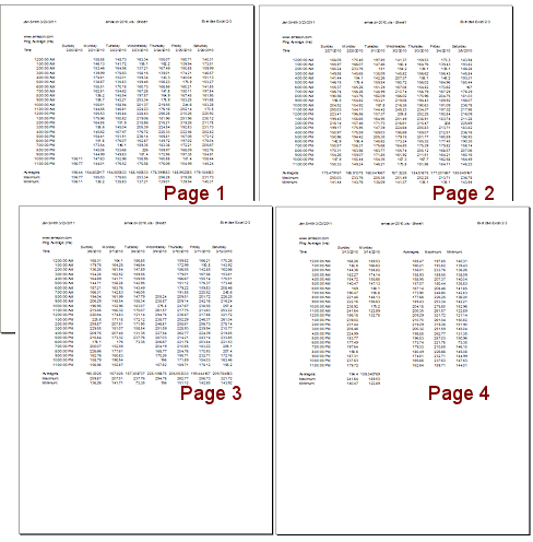
19. Print Preview: Do you have 4 pages? Does each page have the times showing and the titles at the top? Header? Do the rows for Averages, Maximum, and Minimum show on each page? Does the fourth page show the columns for row Averages, Maximum, and Minimum?
    
20. Save.
      [ex2-3-amazon-2010-Lastname-Firstname.xlsx]
21. Print all four pages of Sheet1.