
Jan's Working with Numbers
Format: Arrange: Copy
It would be useful to have the data about each of the special trips on a separate sheet. But no one wants to type all that over again!
There are several ways to copy your data instead of re-typing. Each has different effects and limitations.
-
Drag: You can hold the CTRL key down while dragging to copy a selected range to a new spot on the same sheet. Or you can drag with the right mouse button down to get a context menu that includes Copy. However, you cannot drag non-adjacent ranges at the same time.
-
Copy and Paste: This is usually best when copying to a distant spot on the same sheet or copying to a different sheet. Formulas may need to be corrected.
-
Link: Linking makes a copy that changes whenever the original changes. That method is covered in the next lesson.
| |
Step-by-Step: Copy |
|
| What you will learn: | to copy by dragging range to not drag non-adjacent ranges to copy by pasting on the same sheet to copy by pasting to a different sheet to use Paste Special for Column Widths and All to fix formulas |
Start with: ![]() trips17-Lastname-Firstname.xlsx - Specials sheet (saved in previous lesson)
trips17-Lastname-Firstname.xlsx - Specials sheet (saved in previous lesson)
First you will experiment with copying ranges to new spots on the same sheet. Then you will copy ranges to the new sheets you created in the last lesson. Eventually you will find out how to link the cells so that the pasted cells update automatically when the original data is changed. Powerful!
Each method uses below is good in certain situations. No method is "best".
Copy: Drag Range
You can use the CTRL key while dragging a selection to copy it to another spot on the same sheet. You cannot drag to a different sheet.
- If necessary, open trips17-Lastname-Firstname.xlsx from your Class disk.
-
 Save
As trips18-Lastname-Firstname.xlsx in
the excel project3 folder of your Class
disk.
Save
As trips18-Lastname-Firstname.xlsx in
the excel project3 folder of your Class
disk.
- Click on the tab for the sheet Specials and type A1:F10 in the Name Box and
press ENTER to select the range.
This is the titles, labels, and data for the Tahiti trips. - Hold the CTRL key down and drag the selection by its border
to the right to columns H - M.
The pointer changes to the Copy shape which has a small + beside the arrow.
 If you
don't see the + sign beside the arrow, you will Move the selection rather
than copy it.
If you
don't see the + sign beside the arrow, you will Move the selection rather
than copy it.
-
 With
the CTRL key still held down, drop with the upper left corner at cell H1.
With
the CTRL key still held down, drop with the upper left corner at cell H1.
You may have to drag part of the selection out of the window to get the upper left corner to H1. The window will scroll, sometimes far too quickly!What changed? Not much!
- Column widths were lost.
- Formulas in the last column were adjusted to the new location.
(Click in M5 to see.) That's a good thing!
- Undo since what you
really want to do is to copy this material to a different sheet.
Copy: Drag non-adjacent range?
-
 In the Name Box, type A1:F10, A25:F25 and press ENTER.
The two ranges are selected. Now you are including the Totals row with the Tahiti data. - Try to drag this selection of non-adjacent ranges.
It won't work! Your pointer refuses to change from the Select shape.
You simply cannot drag a selection of non-adjacent ranges.
the Select shape.
You simply cannot drag a selection of non-adjacent ranges.
Copy: Paste
To copy over a distance or to a different sheet, you need to Copy and Paste. This one is just for practice.
Paste to the same sheet
-
 If necessary, select range A1:F10, which contains the titles, column
labels, and Tahiti trips, together with A25:F25, which contains the
Totals.
If necessary, select range A1:F10, which contains the titles, column
labels, and Tahiti trips, together with A25:F25, which contains the
Totals.
A blinking chase lights border appears around both ranges. - Copy.
-
If necessary, scroll horizontally until you can click on cell S1 to select it.
 If using the horizontal scroll bar does not bring S1 into view, click
the scroll arrow at the right end of the horizontal scroll bar to move
further to the right.
If using the horizontal scroll bar does not bring S1 into view, click
the scroll arrow at the right end of the horizontal scroll bar to move
further to the right.Excel can scroll too fast for you at times.
- Paste.
Copy and Paste is much easier than trying to drag the selection this far. No speedy scrolling to try to rein in.
What changed?
- Lost the column widths, which is why the total in cell X11 shows hash marks, #####.
- There is no gap between the rows that were originally not adjacent. But that's probably good!
- Formulas are gone and only values left. May not be good!
Click in X5 and X11 to see what the Formula Bar shows.)
- Undo since you really want this data to be on a different sheet .
Paste to a different sheet
-
 If you have done anything else in Excel besides click on a cell
since you pasted, reselect the ranges A1:F10, A25:F25 and Copy again.Clipboard clears quickly in Excel: Unlike many
other programs, in Excel your copied material is erased from the Windows Clipboard as
soon as you 'do' anything besides move around to find a place to
paste. This is a safety measure! It keeps you from pasting old data by accident.
It is still in the Office Clipboard, which can hold many items instead
of just one thing.
If you have done anything else in Excel besides click on a cell
since you pasted, reselect the ranges A1:F10, A25:F25 and Copy again.Clipboard clears quickly in Excel: Unlike many
other programs, in Excel your copied material is erased from the Windows Clipboard as
soon as you 'do' anything besides move around to find a place to
paste. This is a safety measure! It keeps you from pasting old data by accident.
It is still in the Office Clipboard, which can hold many items instead
of just one thing.To know whether or not the Windows Clipboard still holds what you THINK it does, look for the blinking outline that shows what you copied. If there is no blinking outline, the selection is not on the Windows Clipboard.
Warning:
If you click in the Clipboard task pane to paste your non-adjacent
selection, you will get everything in between also!
- Click on the Tahiti sheet tab to make it the active sheet.
- Click in cell A1 to select it and then paste.
The copied cells are pasted in order, with the non-adjacent rows now adjacent.What changed?
- Lost the column widths, which is why the total in cell F11 shows hash marks, #####.
- There is no gap between the rows that were originally not adjacent. That's good.
- Formulas are gone and only the current values were pasted. Not good!
(Click in F5 and F11 to see.)If you make changes back on the sheet Specials, or if you change values on this table, the totals will not be updated because there is no formula there. This is not usually what you want to happen!
- Undo.
Next you will do this in a way that will preserve the formulas. Drag to
another sheet with ALT: You can drag a selection
to move it to another sheet by holding the ALT key down while you drag over the tabs
until you make active the sheet that you want. Then, continue holding
ALT down while dragging to the destination
cell and drop. This requires a steady hand.
You cannot right drag to copy with ALT. The menu you need pops up and vanishes right away!
Copy: Paste Special Dialog
With Paste Special you have more control over what is pasted. The default choice, All, will attempt to copy formulas. Pasting formulas often causes problems, so be prepared to do repairs.
![]() Clipboard clears quickly! Remember that
the Windows Clipboard will dump your copied or cut data as soon as you do anything
else.
Clipboard clears quickly! Remember that
the Windows Clipboard will dump your copied or cut data as soon as you do anything
else.
-
 On
the Specials sheet, reselect the ranges A1:F10, A25:F25 and Copy again.
On
the Specials sheet, reselect the ranges A1:F10, A25:F25 and Copy again.
- Switch to the sheet Tahiti and select cell A1.
- Click the arrow under the Paste button on the Home
tab and click on Paste Special.
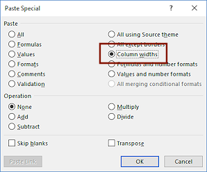
The Paste Special dialog opens.
 Read the list of choices carefully.
'All' does not mean all of the features listed in the dialog! Some of them cannot both happen at the same time, like pasting Formulas and pasting Values. One or the other but not both!
 Problem:
You see a different dialog,
Problem:
You see a different dialog,
If you lose what you copied from the Clipboard, Paste Special may be grayed out. If you somehow copied something else and then choose Paste Special, you may a different dialog, perhaps about pasting a Picture or Bitmap or perhaps about Unicode text or Text.
Solution: Click the Cancel button, select the cells, and try Paste Special again.
 Be
sure All is selected at the top and click on OK.
Be
sure All is selected at the top and click on OK.
What changed?
- Text and formulas were pasted and kept their the formatting.
(Click in F5 and F10 to see.) - Column widths were lost.
- The two Totals formulas show #REF!, which means there in a serious problem with them.
#REF! error: The original formula for
the Total in column D was =SUM(D5:D24).
The new location for the formula is in D11, which is one of the
cells to add up. This is called a circular
reference. Excel cannot add up a set of cells that
includes the cell where the answer goes! The #REF! error also occurs when the formula needs to use cells that you deleted or the cells don't contain numbers anymore.
You will fix the error shortly. First let's do something about the column widths.
- Text and formulas were pasted and kept their the formatting.
- Save.
[trips18-Lastname-Firstname.xlsx]
 Excel 2007 - Fix Column Widths Manually
Excel 2007 does not have quite the same features as Excel 2010. What will work best for Excel 2007 is to paste the column widths first and then the data. Who knew!
-
 On
the Specials sheet, reselect the ranges A1:F10, A25:F25 and Copy again.
On
the Specials sheet, reselect the ranges A1:F10, A25:F25 and Copy again.
- Switch to the Tahiti sheet, select A1 again,
and click the arrow for the Paste button and then on Paste Special.
 Select Column Widths and click on OK.
The widths and backgrounds are pasted but not the data. You lost the previous data, of course.
-
Select A1 again and open Paste Special,
choose All and click on OK.
This time you get the data and the column widths stay put! Hurrah!
Next you will fix the broken formulas in row 13.


 Excel 2010, 2013, 2016 - Fix Column Widths - Paste Column Widths Icon
The Paste button and context menu have icons for various Paste options. These are similar to the choices in the Paste dialog, but not always quite the same! The icons are intended to give a clue as to what they will do. The screen tip that appears when you hover over an icon also helps. But sometimes you just have to try things out to see what does what!
-
 If you have done anything else in Excel besides click on a cell
since you pasted, on sheet Specials, reselect the ranges A1:F10, A25:F25 and Copy
again.
If you have done anything else in Excel besides click on a cell
since you pasted, on sheet Specials, reselect the ranges A1:F10, A25:F25 and Copy
again.
- Click the arrow on the Paste button on the Home tab and click on Paste Special...
- Click on the item for Column widths and then on OK.
Whoops! ALL you got was the formatting and column widths. The cell
contents vanished!
- Undo!!
 Instead
of using the Paste button, right
click on the selection and click on the icon for Column
Widths
Instead
of using the Paste button, right
click on the selection and click on the icon for Column
Widths 
 .
.
The widths adjust to match what you had on sheet Specials.
Hurrah!
Alternate method: Like in Excel 2007, you could use Paste Special to paste the Column Widths first and then paste All.
-
 Experiment: Paste Icons vs. Paste Dialog
Paste Icon: Copy what you succeeded in pasting and paste it in a clear area over to the right using one of the paste icons from the Paste button or right click menu.Paste Special dialog: Then move over to a clear spot and paste again using the Paste Special dialog and the similar paste choice there. Are the results the same? Did you understand what was going to be pasted?
Which icons and commands work the same? Which do not have an exact equivalent in the other method? Which feels more comfortable to you?
When you are ready to continue... Undo all your changes so that the Tahiti material is safely pasted with the column widths correct and the formulas in place.
Next you will fix the broken formulas in row 13.
-
Save.
[trips18-Lastname-Firstname.xlsx]
Fix Formulas
- Click on each of
the totals cells in Column F to see what the Formula bar shows. The
formulas in most of Column F are working fine. But the ones in Row 11
have a problem.
Circular References: #REF! in a cell means that
the cell references in the formula don't work. In cells D11
and F11, the formulas are themselves sitting in cells that are used in the
original formulas. This creates a circular reference,
by trying to calculate using the cell that the formula itself is in. The
cure is to rewrite the formulas.
-
 On
the Tahiti sheet, select cell D11 .
On
the Tahiti sheet, select cell D11 . - On the Home tab, click the AutoSum button
 .
.
The columns above D11 are added, which is what you want.
- Press ENTER.
- Repeat for F11.
- Save.
[trips18-Lastname-Firstname.xlsx] - Experiment: Test the Formulas
Change some of the values on the Tahiti sheet that are used in formulas.
The calculated values should change also.
Undo your changes. - Experiment: Test the Sheets
Change some of the values on the Specials sheet for Tahiti trips.
Check to see if the Tahiti sheet values match. (They won't.) The two sheets are not linked.
Undo your changes! (Key combo CTRL + Z is the same as the Undo button.) Point of Confusion: Your table will now adjust the totals if you change the values on the
Tahiti sheet, but nothing will change on this sheet if you make changes
on the sheet Specials. We will look at how
to make Tahiti update when Specials changes in the next lesson.
Point of Confusion: Your table will now adjust the totals if you change the values on the
Tahiti sheet, but nothing will change on this sheet if you make changes
on the sheet Specials. We will look at how
to make Tahiti update when Specials changes in the next lesson.Be sure to Undo all changes you made with your experiments. (Hint: You saved before you began your experiments. If you now close without saving changes, you can reopen the file to get back to your last saved version.)
|
|
| © 1997-2017 Jan Smith All Rights Reserved |
Site Map What's New |
Privacy Policy Terms of Service Copyright Acknowledgements |
~~ 1 Cor. 10:31 ...whatever you do, do it all for the glory of God. ~~
Last updated: March 22, 2017