
Jan's Working with Numbers
Format: Arrange: Move
It is rather amazing how often you need to move a row or column on your spreadsheet. Fortunately Excel makes this easy to do. You do have to plan ahead, however. If you are not careful, you may overwrite other cells and lose their data.
Animation: Moving a row (loops 5 times)
Refresh
the window to replay the animation.
When you want to shift a row or column without losing the existing data, you must move the existing cells either right or down. Those are the only choices.
Step-by-Step: Move |
|
| What you will learn: | to move by dragging to empty cells to move by cut and paste to move cells to non-empty cells to move with right drag to move with menu commands to move a sheet |
Start with: ![]() trips15-Lastname-Firstname.xlsx - Sheet1 (saved in previous lesson)
trips15-Lastname-Firstname.xlsx - Sheet1 (saved in previous lesson)
Whether you are moving a single cell, a range, a row, or a column, the same methods apply. The method you choose will depend on whether the destination is blank or already has data and on whether you want to replace the data or move it aside to insert the new data.
To practice moving data, you will first move the some columns away from the lower table. Then you will put the table back together again by moving its other columns. You will switch the positions of the Customer and Trip columns in the upper table and then the positions of the Week and Date columns in the lower table. Your final move will be to move the sheet Tickets Sold Chart.
Move: Drag to Empty Cells
- If
necessary, open trips15-Lastname-Firstname.xlsx to Sheet1.
 Save
as trips16-Lastname-Firstname.xlsx to the excel project3 folder on your Class
disk.
Save
as trips16-Lastname-Firstname.xlsx to the excel project3 folder on your Class
disk.
- Select range D27:E37 in the bottom table.
You will move these cells a column to the right.
- Move the mouse pointer over the right edge of
the selection until it changes to the Move shape
 .
.
- Drag the border of the selection to the right.
A border shows where your selection will paste if you release the mouse button.
 When E27:F37 is highlighted in gray (look for the screen tip), release the left mouse button to drop the cells.
All of the formulas still work! You moved all of the cells needed by the formulas.
The cells in D27:D37 are now blank and are not formatted.
Column F is not wide enough to show the whole label.
- AutoFit column F.
(Reminder: Double click the right edge of the Column F header.)
- Save.
[trips16-Lastname-Firstname.xlsx]
Move: Cut and Paste
Next you will cut the rest of the lower table and paste it next to the columns you moved. This only makes sense for practice! Normally you would have moved or cut and pasted the whole table at once.
-
 Select range A27:C37 and cut it by clicking
 the Cut button or use the key combo CTRL + X.
 The selected range gets a blinking border.
- Select cell B27, which will be the upper left cell for
the new location.
- Paste with
 the Paste button or use the key combo CTRL + V.
- Click out of the table to deselect.
When you pasted, you pasted both the cell contents and the formats. The now-empty cells in column A have lost their formatting. So cool!
- Save.
[trips16-Lastname-Firstname.xlsx]
Move: Drag to Nonempty Cells
Now we get more complicated. When you start to drop cells on top of cells that already have contents, Excel needs to know what to do with the existing data - dump it or move it.
You are going to revise the table so that the Trip column is at the left and the column Customer is next to it on the right.
-
 If
necessary, click in a blank cell to deselect what you pasted and scroll
up to see row 4.
If
necessary, click in a blank cell to deselect what you pasted and scroll
up to see row 4.
- Select range A4:A25, which is the column of Customers
in the first table. You want to move this to the right so that it is
between the columns for Trips and Number of People.
- Move the mouse pointer over the right border of your
selection. The pointer changes to the Move shape.
-
 Drag the selection by its border to the right until the range B4:B25 has its border highlighted.
Release the mouse button.
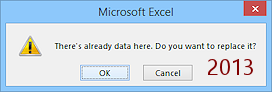 Instead of the cells being dropped, you get a message asking if you want
to replace the contents of the destination cells. No! You don't want to
do that. No other choices are offered. Not very friendly!
Instead of the cells being dropped, you get a message asking if you want
to replace the contents of the destination cells. No! You don't want to
do that. No other choices are offered. Not very friendly! - Click on Cancel since you don't want to erase any
data.
The selection goes back to its original place, but it is still selected.
Move: Right Drag
Dragging another way will give you more options for what Excel can do.
-
 Right
drag (Hold the right mouse button down while dragging) the selection by the border to the right until the range B4:B25 has its border highlighted.
Right
drag (Hold the right mouse button down while dragging) the selection by the border to the right until the range B4:B25 has its border highlighted.
-
Release the mouse button.
A context menu appears with many choices.You want the selected data to move to the right.
-
Click on Shift Right and Move.
Whoops. Nothing happened!The Shift commands will move what is currently in the destination cells, the Trips cells. But none of the choices will shift the Trips cells to the left where you want them! Only right and down are available. Rats! You will have to do this another way.
Clearly you must plan how you are going to drag cells so that the existing data can shift right or down. Let's try moving the Trips column instead of the Customer column.
- Select range B4:B25, which is the Trips column.
- Right drag to the left until the range A4:A25 has its border
highlighted. Release the mouse button. The context menu appears
again.
-
 Select Shift Right and Move.
Hurrah! The Trips cells are moved to the left and the Customers cells are shifted right. Just what you wanted.The column widths did not change to match the new contents.
- AutoFit columns A and B by double-clicking the
right edge of the each of the column headings.
- Save.
[trips16-Lastname-Firstname.xlsx]
Move: Cut and Insert with Menu
Another way to move data to a new spot is to Cut it and then Insert what you cut. Pasting would overwrite data that was already there. Inserting moves existing data out of the way, and you get to choose which direction.
-
 Select range C27:C36, the Date column in the second table.
You want it to switch places with the Week column. That is, you want to insert the selected data and move the Week data over to the right. But you need to leave the word Totals: in place.
- Cut with the Cut button on the Home ribbon tab or the key combo CTRL + X.
The selected range now has a blinking border. If you
press ESC now, your data is not cut after all and the blinking border is
removed.
If you
press ESC now, your data is not cut after all and the blinking border is
removed.
- Right click on cell B27, the top of the Week column.
-
 From
the menu select Insert Cut Cells .
From
the menu select Insert Cut Cells .
The Date column is now on the left, followed by the Week column. Excel made a guess as to what you wanted to do after removing the cells that you cut. It was right! - If necessary, press the ESC key to remove the blinking border.
 If
you copy cells (instead of cut), when you paste, you get a list of
choices for what you can do.
If
you copy cells (instead of cut), when you paste, you get a list of
choices for what you can do.
-
 Save.
Save.
[trips16-Lastname-Firstname.xlsx]
- Switch to Print
Preview.
This may take two sheets right now, depending on the default margins of your version of Excel.
- If necessary, set Scaling to fit on one page in Portrait orientation.
-
 Print
Print
- Close Print Preview.
Move: Sheet
Excel 2007 and 2010 include 3 blank sheets in the blank document template. Excel 2013 and 2016 only have one. Your workbook now has at least two sheets. To practice moving, you need at least three.
When you create a new blank sheet, it will have a default name like Sheet3 or Sheet4. The number will depend on how many sheets you have created during this editing session, even if you deleted them.
-
If necessary, create a new blank worksheet so that you have at least three worksheets.

 Excel 2007, 2010: Click on the New sheet tab
  to the right of the sheet tabs. A new sheet tab appears.
 Excel 2013, 2016: If necessary, click the tab Tickets Sold Chart to select it. Click the New sheet button
  on the Status bar to the right of the sheet tabs. A new sheet tab appears to the right of the currently selected tab.
 Drag the tab for the sheet Tickets Sold Chart to the right.
A small black arrowhead appears above the sheet tabs and the pointer now includes a sheet of paper icon.
-
 When the arrow is at the far right of the last sheet tab, release the mouse button to drop the sheet.
  Experiment: Moving sheets
Practice dragging the sheet tabs to change the order.
- Save.
[trips16-Lastname-Firstname.xlsx]
|
|
| © 1997-2017 Jan Smith All Rights Reserved |
Site Map What's New |
Privacy Policy Terms of Service Copyright Acknowledgements |
~~ 1 Cor. 10:31 ...whatever you do, do it all for the glory of God. ~~
Last updated: March 22, 2017