
Jan's Working with Numbers
Formulas: Changes: Inserting
Sometimes inserting rows and columns causes formula problems and sometimes it does not. What makes the difference is where you are inserting and what the formula range includes.
Where you insert makes a difference:
- Inside the range: All is well. Excel understands that the new cells inside a formula's range are supposed to be included in the results. Excel adjusts the formula for you.
- Completely outside the range: Of course you don't expect the formula to include this data, and it doesn't!
- At the edge of the range: The formula may not use those cells. It depends on which edge and whether or not the formula's range included blank rows.
| |
Step-by-Step: Inserting & Formulas |
|
| What you will learn: | to insert row without breaking formula
to fix a formula broken when cells were inserted |
Start with: ![]() trips28-Firstname-Lastname.xlsx (saved in previous lesson)
trips28-Firstname-Lastname.xlsx (saved in previous lesson)
After you have gotten your worksheets all fixed up and formatted, you find that you have omitted some trips. Whoops! You need to insert some more trips on the sheet Specials. Since rows and columns behave the same, you can learn about handing this kind of problem by looking at the what happens to rows.
You will find out what happens when you insert...
- inside range
- at the bottom border of range with blank row
- at bottom border of range without a blank row
- at top border
Insert Row: Inside Range
The first new trip to add is to New Zealand, sold by Gardner to Midland Associates for 5 people. (He must be a good salesman to sell them a second trip so soon!)
You need to put this information in the middle of the table between rows 14 and 15.
- Open trips28-Firstname-Lastname.xlsx from your Class disk in the folder excel project4.
-
 Save
As trips29-Lastname-Firstname.xlsx in the excel project4 folder of your Class
disk.
Save
As trips29-Lastname-Firstname.xlsx in the excel project4 folder of your Class
disk. 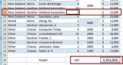 On
the sheet Specials select row 15.
On
the sheet Specials select row 15.- Right click on the selection and in the context
menu, click on Insert.
A new row appears above the selected row. - Copy the information in the first 3 cells of the row 14 into
the new blank row and .
[Hint: use the key combo CTRL + ', which is a single quote, usually found near the ENTER key on a key with ", double quote, also.]
- In the Number of People column enter the number 5.
What changed?
- In the new row Total sale shows up automatically, $15,000.
Excel assumes you want to use the same type of formula for this row as for the surrounding rows. Smart!
(If the formula does NOT automatically appear, copy the formula from another cell into F15.)
-
The Totals for the table in cells D26 and F26 are larger than before. They automatically included values from the new row.
The ranges of the formulas changed to include the inserted row and plus all the original rows.
The new row was inside the range of the original formula: =SUM(F5:F24). Cool!
- In the new row Total sale shows up automatically, $15,000.
- Save.
[trips29-Lastname-Firstname.xlsx]
Insert Row: At Bottom Edge of Range (Inside Range)
The second trip to be added is in the Other category
-
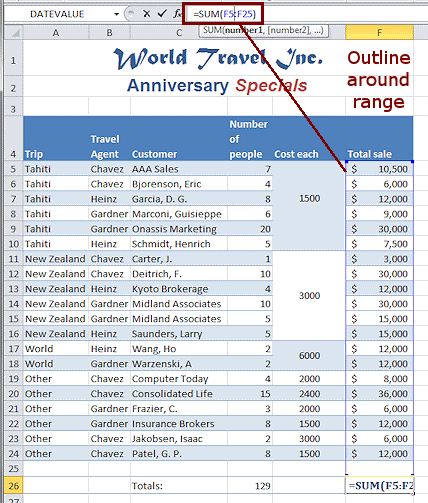 Select cell F26 and inspect its formula =SUM(F5:F25).
This formula includes the blank row 25 below the last Total sale value. -
Click in the Formula bar inside the formula.
A colored outline surrounds the range that the formula uses. Drag outline handles: The
colored outline has handles at the corners that you can drag to
change the range. This is a quick an easy way to correct some kinds of errors in
a formula.
Drag outline handles: The
colored outline has handles at the corners that you can drag to
change the range. This is a quick an easy way to correct some kinds of errors in
a formula. - Press the ESC key to get out Edit mode for the formula.
- Select row 25 and insert a row.
A new row appears, using the formatting from the row above, row 24.
We don't want that formatting!
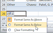 Hover over the Format Options button below your new row and
click the arrow.
Hover over the Format Options button below your new row and
click the arrow.- Select Format Same As Below.
This options button is a big help... unless neither the row above nor the row below is quite what you want. -
 In
the new row 25 enter the following:
In
the new row 25 enter the following:
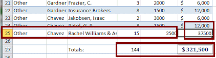
Trip: Other
Travel Agent: Chavez
Customer: Rachel Williams & Associates
Number of People: 15
Cost each: $2500Again, the Total sale formula automatically calculates and the Totals for the table includes the new values. The new row wound up inside the formula's range for both Totals. This is working out pretty easy!
But wait... the formatting is wrong for E25 and F25.
Recall that you chose Format Same As Below. The row below was a blank line. You may have included that row when you applied formatting and maybe not! -
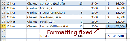 If
necessary, select cells E23:F23 and copy their formatting to E25:F25.
If
necessary, select cells E23:F23 and copy their formatting to E25:F25. (You know more than one way to do this. You can do it manually, use Format Painter, you can Copy and Paste Formats, or use AutoFill > Formatting only.)
Why did we use E23:F23 instead of the row right above, E24:F24 to copy the formatting? In row 23 the background is white. In row 24 it's blue!
- Save.
[trips29-Lastname-Firstname.xlsx]
Insert Row: At Bottom Edge of Range (Outside Range)
You will add the third trip to the Other category also, but outside the range of the Total for the whole table. This row is between the data and the cell with the formula and there is no blank row.
- Delete the blank row 26.
- Inspect the formula in F26, which now shows =SUM(F5:F25).
There is no blank row. - Select a cell in row 26 (which is now the Totals row) and insert a
new row.
It appears above the selected row and has the formatting of the row above it. - Inspect the formula in F27, which shows=SUM(F6:F25).
It does not include the row you inserted at the bottom edge of the formula's range. - Add the following information to row 26:
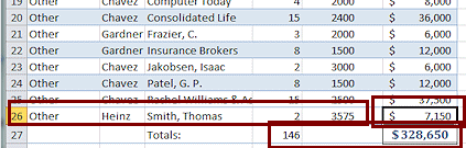 Trip: Other
Travel Agent: Heinz
Customer: Smith, Thomas
Number of People: 2
Cost each: $3575Excel automatically inserts the formula for column F in this row and updates the Totals in row 27. Hurrah! Older versions of Excel did not do this.
- Save.
[trips29-Lastname-Firstname.xlsx]
Insert Row At Top Edge of Range (Outside Range)
-
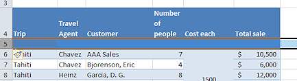 Select row 5 and insert a new row.
It appears above the selected row but with the formatting of the columns labels. Not a good guess by Excel!
The Formatting Options button won't help. We don't want to use the formatting from either the row above or the row below. - Reformat row 5: Select E5 and the merged cell E6. Click the Merge & Center button.
The original merging is removed. Click Merge & Center again.
Now E5:E11 merge. - Use Format Painter to copy the formatting of the other cells in row 7 onto row 5.
-
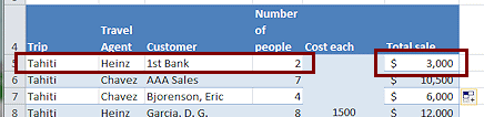
 Add the following information to row 5:
Trip = Tahiti
Travel Agent = Heinz
Customer = 1st Bank
Number of People = 2
[Cost each is already in the merged cell]The Total sale is not calculated. The totals in row 28 do not change.
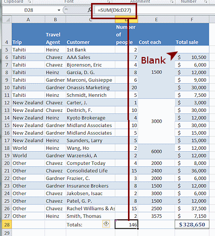
- Click in cell D28, the total for
the number of people.
The formula does not include row 5. The same is true for cell F28, the total for sales.
It's back to the repair shop for the totals formulas.
- Save.
[trips29-Lastname-Firstname.xlsx]
Fix Broken Formulas
-
 AutoFill from cell F6 to F5.
Now the Total sale is calculated, but the Totals at the bottom in row 28 still do not include row 5.
- Use the AutoFill Options button to Fill Without Formatting.
- Click in cell D28 and then in the formula
bar click on the range.
A colored outline surrounds the cells D6:D27. 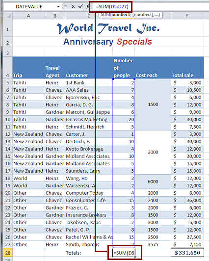 Drag the handle of the colored outline up to include
row 5.- Click the check mark button.
Now the formula uses the range D5:D27, which is correct. - Similarly, repair the formula in F28 to include row 5.
- Save.
[trips29-Lastname-Firstname.xlsx]
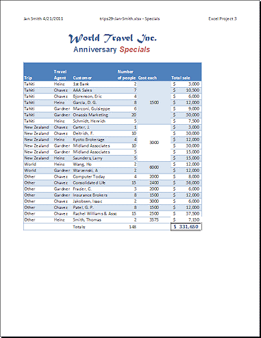
- Select the upper table on the sheet Specials [A1:F28].
-
 Print the selection.
Check Links on Other Sheets
You added four rows to the original data for 1st Bank, Midland Associates, Rachel Williams & Associates, and Thomas Smith. Did any of your sheets with linked cells pick up the new data?
-
Select each of the other sheets in turn and look for changes.
Only one sheet shows a change. The sheet Formatted Groups does not show the new rows but does show the new totals in D28 and F28 on the sheet Specials. Those cells were linked directly to the Specials cells.
Linking cells does not link ranges, just individual cells. The new rows do not show up on the sheets with linked cells. You would have to Paste Link all over again to update the other sheets.
We also have not updated the lower table with new values for the sales in each week.
Since this is not the "real world", we can save you some effort and let those sheets stay as they are. Broken!
Conclusions about Inserting
- Inserting rows and columns inside a formula's range updates
the formula automatically.
- Inserting a row or column at the bottom or right edge of a
range should update the formula. You must check to see if it did.
- Inserting a row or column at the top or left edge of a range will not update the formula.
- Inserting rows and columns does not update other sheets with the new rows/columns. A total cell that is linked to the original will update.
|
|
| © 1997-2017 Jan Smith All Rights Reserved |
Site Map What's New |
Privacy Policy Terms of Service Copyright Acknowledgements |
~~ 1 Cor. 10:31 ...whatever you do, do it all for the glory of God. ~~
Last updated: March 22, 2017