Jan's Working with Numbers

Step-by-Step: Flash Fill Data

---

What you will learn:

to apply Flash Fill automatically to apply Flash Fill manually to use Flash Fill on column adjacent to data to use Flash Fill on column NOT adjacent to data to use Flash Fill to combine data to use Flash Fill to split data

---

Start with: flashfill.xlsx from the resource files

Warning: Type accurately. Flash Fill will not see a pattern if you mis-type the data!

To get some practice, you will use a resource file instead of the sheet on trips for World Travel Inc.

Apply Flash Fill Automatically

When typing in a lot of text, it is easy to get the capitalization or spacing messed up. Flash Fill can help with that, but you must create a new column for the revised data.

1. Open the file flashfill.xlsx from the resource files.

2. Save as
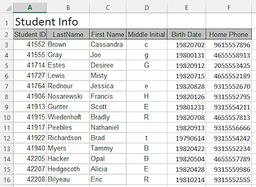
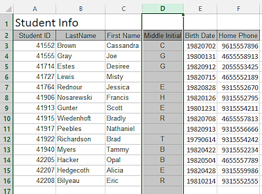
   flashfill-Lastname-Firstname.xlsx to the excel project2 folder of your Class disk.

   Notice that Column D has some lower case and some upper case. For these few it would be easy to retype. But suppose there were 3000 records to inspect and fix. Flash Fill was made for just this kind of situation.

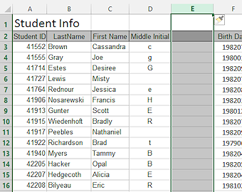3. Select Column E by clicking its header.
4. Right click the selection and click on Insert.
   One blank column appears to the left of the selected column. However many columns are selected is how many will be inserted.
5. In cell E2 type a column heading Middle Initial and press ENTER.
   Now two columns have the same heading. That's OK. You will be removing one of the columns shortly.
   
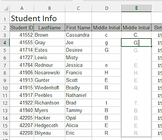6. In E3 type the letter C as an upper case letter and then a period, C.
7. Press the ENTER key to accept your typing and move the selection down one cell.
8. In E4 type an upper case G .
   If you wait briefly, Flash Fill pops up a preview of its suggestions before you even type the period.

9. Press the ENTER key.

   All of the suggestions are accepted.

   Alternate Method: Click on the check mark button on the formula bar. Your typing is accepted but the selection does NOT move.
   

10. Inspect the new Middle Initial values.
    There is a period when there was no middle initial in the original columns. Interesting but odd. There is another way to get what we want.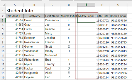

11. Select cells E3:E16 and press the DELETE key.
    The cells are blank now.
12. Save.
    [flashfill-Lastname-Firstname.xlsx]
    

---

Apply Flash Fill Manually - Flash Fill Button

Sometimes Flash Fill does not show you a preview list or the list vanishes before you can accept the suggestions. On the Data ribbon tab, the Flash Fill button will become active (no longer grayed out) once Excel is ready to guess what the pattern is.

For some reason Flash Fill understands what you just did with the upper case letter followed by a period better than with no period. This will give you a chance to use the Flash Fill button.

1. Click in cell E3 to select it.
   This is the first cell in a blank column.
2. If necessary, click the Data ribbon tab to show its buttons.
3. Find the Flash Fill button in the Data Tools tab group.
   The button is active! What suggestions do you think it will make?

4. Click the Flash Fill button.
   The values in the original column are duplicated. This could be useful in the right situation but not this time.

5. Undo.

   Now we can try to get Flash Fill to make changes.

6. In cell E3 type C . (without a period)
   The Data ribbon goes gray. None of the tools are available while you are editing.
7. Press ENTER.
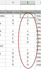
   The tools are back, including Flash Fill. But you did not get a list of suggestions.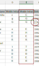
8. On the Data ribbon tab click the Flash Fill button .
   There is no preview but the rest of the column is filled in.
9. Inspect the new values.
   Where cells in the original column were blank, the new cells are blank. Hurrah! This is what we were looking for this time - all caps and no periods and preserving empty cells.
10. Select Column D which holds the original middle initials.
    

11. Right click on the selection and click on Delete.
    The column is removed.

    Warning: DELETE Key vs. Delete Command
    The DELETE key removes the contents of the cell but leaves the column in place.
    The Delete command removes the whole column.

12. Save.
    [flashfill-Lastname-Firstname.xlsx]

---

Use Flash Fill with Column Adjacent to Data

Phone numbers do not behave like numbers since you cannot do arithmetic with them. So data cells for phone numbers should be formatted as Text or General.

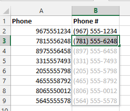
Phone numbers can be formatted in several different ways, like 345-555-3214 or (345) 555-3214 or 345.555.3214. Flash Fill can make it easy to change the way your spreadsheet displays a phone number, no matter how many rows of records you have.

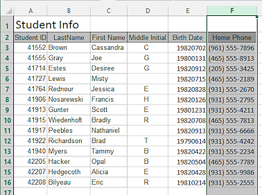
You will format the phone numbers with parentheses in a column directly beside the data column. Those characters are text. These numbers are fiction, of course. In the USA numbers with 555 in the middle are never assigned to real people or businesses. This allows books, movies, TV shows (and computer lessons!) to use these 555 numbers without having to worry about whose phone number it really is. So smart of someone to think of doing that!

1. Copy and paste cell F2 to cell G2.
   This creates a column heading for column G, which is blank.
2. Select Column G by clicking its header.
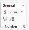3. On the Home ribbon tab verify that the data type is General.
   Flash Fill does not automatically format numbers.
   
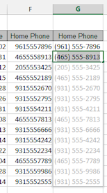4. In cell G3, type the phone number that is in F3 but include punctuation, like (961) 555-7896 .
   Note - there is a space after the second parenthesis.
5. Drag the right edge of the header for column G to make the column's width 96 pixels.
   This will make the column wide enough to show the phone number in its new form.

6. In cell G4 start to type the phone number that is in F4.
   As soon as you type the first parenthesis, Flash Fill shows a preview of its suggestions. The parenthesis is a text character so Flash Fill knows it is allowed to make a guess.

   Problem: Flash Fill did not provide suggestions
   Solution: Type the next phone number in cell G5. Flash Fill needed more data to create a pattern. Excel 2016 does this.
   

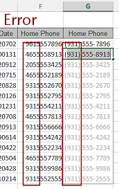   Problem: All area codes are the same
   This is an example of the kind of error that can occur when you have done a lot of entering, editing, and/or deleting in the column. Flash Fill has gotten confused.

   Solution 1: Keep typing characters in your second example. You may have to use the Flash Fill button on the Data ribbon tab to get the suggestions.

   Solution 2: Delete the revised numbers and start over. Be sure the cells have General format.
   

7. Press the ENTER key to accept all of the suggestions.
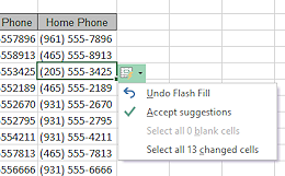
   The rest of the rows are filled in with the same format.

   An Options buttons appears near the third cell of data.

8. Click the Options button to open its menu of options.
   You could undo what you just accepted. You can select blank cells that Flash Fill fails to populate. You can select all of the changed cells to do more formatting on all of them at once.
9. Click on a blank cell to close the menu.
   
10. Select column F, which holds the original phone numbers.

11. Right click on the selection and choose Delete.
    The column vanishes and Column G moves left to become the new column F.

12. Save.
    [flashfill-Lastname-Firstname.xlsx]

    
    

---

Flash Fill with Column NOT Adjacent to Data

The data column(s) you are using with Flash Fill do not have to be directly next to the blank column. But they do need to be within the data range or adjacent to it. Let's try another version of the phone number in a different column to show this.

Blank Columns between Data and Flash Fill Column

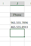1. In cell J2, type Phone # as a column heading.
   This leaves some blank columns between the data range and column J, the target column for Flash Fill.
2. In cell J3 and type the phone number 961.555.7896 and press ENTER.
3. In cell J4 type the next phone number as 465.555.8913 .
4. In cell J5 type the next phone number as 205.555.3425
   Flash Fill does not offer suggestions.

5. On the Data tab, click the button Flash Fill .
   A message appears instead of suggestions. Flash Fill does not see a pattern. The data range is too far away.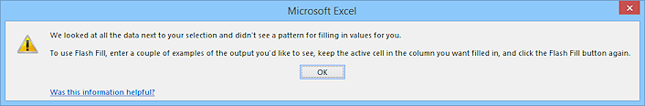

   

6. Delete the column.

Blank Column for Flash Fill Inside Data Range

Next you will insert a blank column that is inside the data range, but it is not adjacent to the data that it is using for Flash Fill.

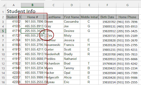
1. Insert a new blank column between the columns Student ID and LastName.
2. Type Home # as a new column heading in column B.
3. Type in cell B3 the phone number with periods between the parts, like
   961.555.7896
4. Press ENTER.
5. Widen the column enough to show the whole number by dragging the right edge of the B header to the right.

6. In B4 type the phone number as 465.555.8913 and press ENTER.
   FlashFill does NOT provide suggestions. Apparently with this arrangement. FlashFill thinks you are typing numbers. FlashFill does not work for numbers.

   Or Flash Fill may offer a format with the first five numbers followed by #. That pattern would be from including the header, Home #.

7. If necessary, click on the Data ribbon tab.
   The controls on this tab should be available, including Flash Fill.

8. Click on the Flash Fill button.
   The cells are filled in by Flash Fill without the 'preview' showing first.
   The Flash Fill Options button shows up so you can change your mind if the entries are not what you wanted.
   

   Problem: Flash Fill error message - No pattern

   

   Solution 1: Inspect the examples that you entered and make sure that you typed correctly!
   If you mistyped a character, Excel will not be able to figure out the pattern. Make corrections and try the button again.

   Solution 2: Enter more examples to more clearly show Excel what the pattern is.
   In this exercise Excel should not need more examples but in other situations three or even four examples may be necessary to make the pattern clear.

9. Save.
   [flashfill-Lastname-Firstname.xlsx]

---

Use Flash Fill to Combine Data

Sometimes you want to see a complete name instead of parts of a name. Flash Fill can put the parts together for you. If some records are missing a part, a second effort by Flash Fill can help.

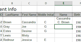1. Insert a blank column to the right of the Middle Initial column.
2. Type Name in the heading for the new column and press ENTER.
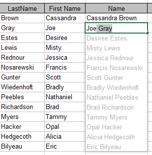
3. In cell E3 type Cassandra C. Brown and press ENTER.
   The text wraps to the cell width and the row gets taller to hold the full name.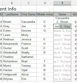
4. Similarly, start typing the next name in E4, Joe G. Gray.
   Flash Fill quickly offers suggestions before you type much at all.
   
5. Press ENTER to accept all suggestions.
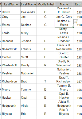
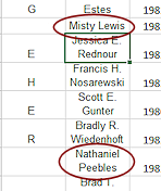
   The cells get taller to show the wrapped text.
6. Inspect the names that did not have a middle initial.
   They have a period between the first and last names. Misty . Lewis and Nathaniel . Peebles. Not a good look!
7. Click in cell E7, Misty . Lewis.
8. Edit the name to remove the period and one space.
   

9. Click the check mark button on the Formula bar or press ENTER.
   The period is automatically removed from the other instance, Nathaniel Peebles. Sweet!

10. Save.
    [flashfill-Lastname-Firstname.xlsx]

---

Use Flash Fill to Split Data

Sometimes your data comes to you in a combined form when you need to sort or group it on a part. Flash Fill may be able to help out, if your data is similar enough throughout the column. You cannot use Flash Fill on two or more columns at once. You must handle each part that you are splitting off separately.

In this section you will split the new Name column back into separate columns. What will Flash Fill do with the names that only have two parts?? Let's see!

1. Select columns C, D, and E - LastName, First Name, Middle Initial.
2. Press the DELETE key to remove the text.
   Now the only name information you have is in the Name column. We can be sure that Flash Fill is looking at the Name column.
3. Type headings in row 2, First, Middle, Last.
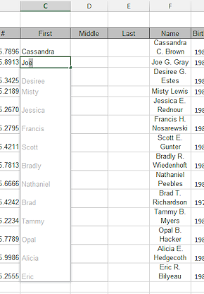
4. Type in cell C3 the first name Cassandra.
5. Type in cell C4 the first name Joe.
   Flash Fill offers suggestions for the rest of the column.

6. Press ENTER to accept the suggestions.

   Tip: Suggestion List Vanished
   If you lose the list of suggestions before you can press ENTER, go to the Data ribbon tab and click on the Flash Fill button. If that button is grayed out, use ENTER or the down arrow to move to a blank cell in the current column. The button should become available.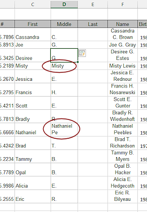

7. In cell D3 type the middle initial with its period, C.

8. In cell D4 type the middle initial G.
   Flash Fill offers suggestions, including something unexpected for the two names that do not have a middle initial.

   It is not clear what pattern Excel thinks that it has found!

9. Press ENTER to accept the suggestions anyway.
10. Click in cell D6 and delete the text, Misty.
11. Press ENTER.
    The other odd entry did not change.
12. Delete the contents of cell D11, Nathaniel Pe.
    

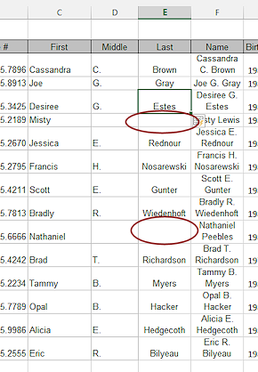13. Similarly, use Flash Fill to fill in column E, Last.
    Whoops. Two last names are missing.

    Problem: Flash Fill does not offer suggestions; Flash Fill button suggestions are wrong
    Solution: Delete Column E completely and insert a fresh column. Type in the title, Last, and try again.
    

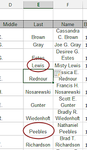14. In cell E6, type Lewis.

15. Press ENTER.
    Peebles is also filled in in row 11.
    All last names are properly in place!

16. Save and Close the spreadsheet.
    [flashfill-Lastname-Firstname.xlsx]

    From these few examples, you can see how helpful Flash Fill can be but also how careful you must be to inspect the results.