
Jan's Working with Numbers
Excel Basics: Arrange: Rows
Like columns, you can apply formatting to a whole row or several selected rows at once - font, font size, font color, bold, italics, and such. The only formatting that is unique to rows is Row Height. Row Height is measured in points, like font size, from 0 to 409 points. You will work with text formatting choices in the next project. For right now, let's look at row height.
![]() Tip: A row height of zero hides the row.
Tip: A row height of zero hides the row.
The default setting for Row Height is AutoFit. The row height adjusts to hold the tallest text in that row. The AutoFit row height allows for white space between the text and the cell's border on all four sides, called cell padding.
Examples of Row Height with AutoFit
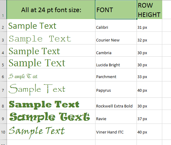
What differences do you see in the examples, besides the shapes of the letters and the AutoFit row height? All are at 24 pt font size to make differences easier to see.
- Which has the most white space above?
- Which has the most white space at the left?
- Which has the least white space at the bottom?
- Which has the largest space between words?
- Which creates the tallest row?
- Which creates the shortest row?
| |
Step-by-Step: Format Rows |
|
| What you will learn: | to adjust row height with AutoFit and font size to adjust row height by dragging row heading to adjust row height with Row Height dialog to adjust row height for multiple rows by dragging to adjust row height for multiple rows with AutoFit to hide a row to unhide a row |
Start with: ![]() trips3-Lastname-Firstname.xlsx (saved in previous lesson)
trips3-Lastname-Firstname.xlsx (saved in previous lesson)
Row Height: AutoFit
You will take advantage of the automatic resizing as you change the font size for the title.
-
 Save
As trips4-Lastname-Firstname.xlsx on
your Class disk in the folder excel project2.
Save
As trips4-Lastname-Firstname.xlsx on
your Class disk in the folder excel project2. -
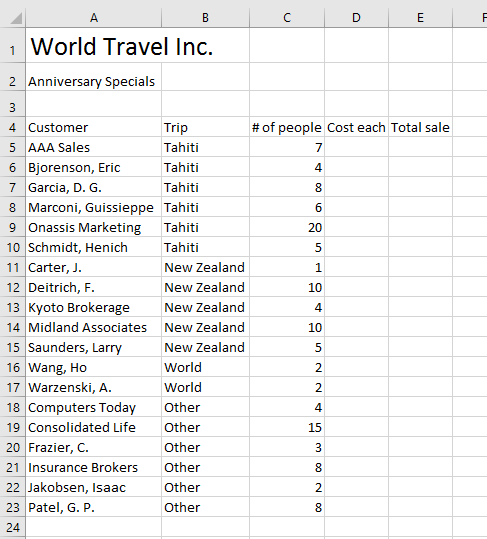
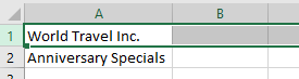 Select Row 1.
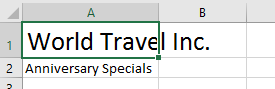 On the Home ribbon tab, use the Font Size control to change the Font Size to 20.
AutoFit automatically increases the row's height.You don't have to change the height of the whole row to get the same effect. Increasing the font size of a single character in a cell in the row will work, too. AutoFit will increase the Row Height to match. Let's prove that.
- Double-click cell A1. You can now edit.
-
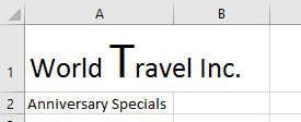 Select a single letter and apply Font Size
36 to it and click on a different cell.
Select a single letter and apply Font Size
36 to it and click on a different cell.
The row height changes for the whole row. Even blank spaces have a font size.
If you have a height error that you cannot find, look at spaces and blank
cells in the row.
Even blank spaces have a font size.
If you have a height error that you cannot find, look at spaces and blank
cells in the row.
- Undo.
The font size for cell A1 is back to 20 points again. -
Save.
[trips4-Lastname-Firstname.xlsx]
Row Height: Drag
-
 Position the pointer over the bottom edge of the Row 1 heading until it changes to
  the Resize Row shape.
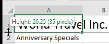
- Click and hold to see the screen tip with the Row Height, 26.25 (35 pixels).
- Release mouse button.
Notice that the Row Height 26.25 is larger than the Font Size that you set to 20 points. This creates the white space around the text. The larger the font size of the text, the more white space surrounds the text in the cell.
If you drag by accident, you will resize the row height. Use Undo to reverse this, if necessary.
- Select Row 2.
-
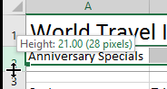 Position the pointer over the bottom edge of the Row 2 heading until it changes to the Resize Row shape.
- Drag downward until the screen tip shows a Height of 21.00 (28 pixels).
- Release the mouse button.
The text is at the bottom of the cell, which is now taller. - Save.
[trips4-Lastname-Firstname.xlsx]
Row Height: Dialog
- Select Row 3, which is blank.
-
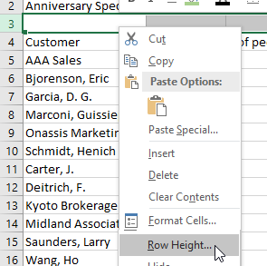 Right click on the selected row and from the
context menu select Row Height...
Right click on the selected row and from the
context menu select Row Height...
The command is also on the Format menu: Home tab > Cells tag group > FormatThe Row Height dialog appears.
-
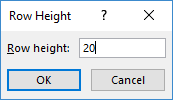 Type in a new height of 20 and click on OK.
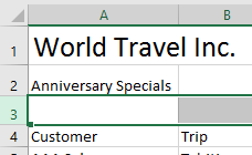
Row 3 is now taller.
-
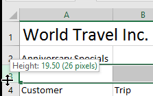 Click on the bottom edge of row 3 to see the row height in a screen tip.
The height is 19.50 points (26 pixels) instead of 20.00 points! What happened?? -
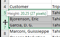
Drag the bottom edge of row 3 down. Watch the pixels change.
26 pixels is 19.50 but 27 pixels is 20.25.You cannot set the row height to exactly 20 points. A pixel is the smallest dot on the screen. The screen cannot show a fraction of a pixel! The dialog did not warn us that a setting of 20 points would not come out exact.
Leave row 3 at 19.50 points (26 pixels).
- Save.
[trips4-Lastname-Firstname.xlsx]
Row Height: for Multiple Rows
-
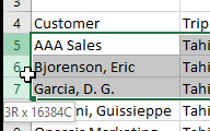
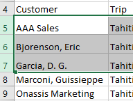
 Select Rows 5, 6,and 7 by dragging across the row headings.
While you drag, a ScreenTip shows how many rows you are selecting, either like 3R or like 3R x 163840. That can be very helpful when you are trying to select a large number of rows!
- While the three rows are selected, move the pointer over the bottom edge of any one of the selected rows until it changes to the Resize Row shape.
-
 Drag downwards until the ScreenTip shows a height of 20.25 points.
 Confusing effect: As you drag, the row headings resize but the rows do not until you release the mouse button.
-
 Release the mouse button.
All selected rows now have the same new height.
Row Height: AutoFit Multiple Rows
The spacing you just created will make the sheet too big if applied to all rows. You should return the rows to the AutoFit height. (Yes, Undo would work here, but you are practicing with Row Heights!)
- Select Rows 5, 6, and 7 again, if necessary.
-
 Double-click the bottom edge of any one of the selected rows.
The rows return to their AutoFit height. - Save.
[trips4-Lastname-Firstname.xlsx]
Hide/Unhide Rows
 Sometimes you want to temporarily hide some rows to make the sheet easier to
read. Or perhaps you have calculations in cells that you don't really need to
see at all because they are just used in other calculations.
Sometimes you want to temporarily hide some rows to make the sheet easier to
read. Or perhaps you have calculations in cells that you don't really need to
see at all because they are just used in other calculations.
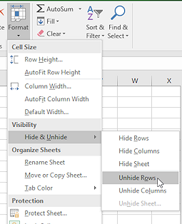
You can hide or unhide rows using the Hide or Unhide command on the menu from the Format Cells button or from a right click menu. Or, you can drag the headers or set the row height to zero to hide. Hiding is easier than unhiding! To reveal the hidden rows, you must first find them and select them. Then Unhide will reveal the rows again or you can set a new row height or use AutoFit to do that. So many ways to do things!
These same procedures work with columns, too.
Hide: Right Click Menu
-
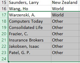
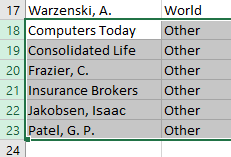 Select rows 18 through 23.
These are trips that were not one of the special anniversary offers.
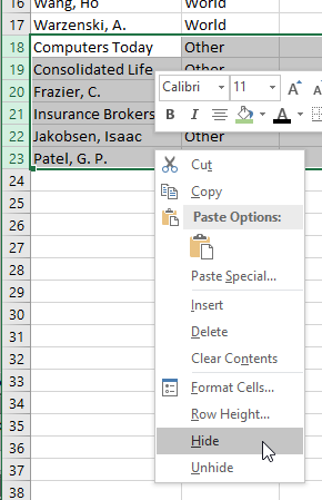 Right
click on the selection and click on Hide.
Right
click on the selection and click on Hide.
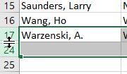
Your selected rows vanish! Notice how the numbers skip now in the row headings from 17 to 24. Sneaky!

 Excel 2007, 2010: The only clue that rows are hidden is that the numbers skip.

 Excel 2013, 2016:
New feature - A gap shows between headers when there are hidden rows.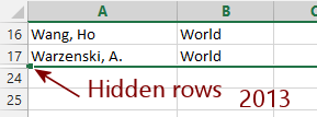
When the mouse pointer is over this gap, the shape changes from the normal Resize Row shape
 to one with a two lines
  , Resize Hidden Rows. What you do while the pointer is in this shape applies to all of the hidden rows.
To make hidden rows appear again is a bit trickier. You cannot select just these rows since they are out of sight. There is no menu command for selecting particular rows.
Unhide: AutoFit
-
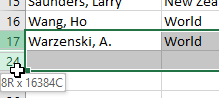 Drag from row 17 to row 24, selecting the whole rows.
You have also selected the invisible rows in between: 18 through 23.
Note the number of rows in the screen tip while you are dragging.Alternate method: In the Name box, type 17:24 and press ENTER.
-
 Double-click the bottom edge of the row headings in your selection.
AutoFit returns all rows to the default height. Whew!Alternate method: Right click the selection and choose Unhide from the context menu.
- Save.
[trips4-Lastname-Firstname.xlsx]
You did make some changes to keep at the top of the sheet.
|
|
| © 1997-2017 Jan Smith All Rights Reserved |
Site Map What's New |
Privacy Policy Terms of Service Copyright Acknowledgements |
~~ 1 Cor. 10:31 ...whatever you do, do it all for the glory of God. ~~
Last updated: March 22, 2017