
Jan's Working with Numbers
Excel Basics: Arrange: Columns
You can apply almost every kind of formatting to whole columns at once. Just select the column(s) and apply the formatting. This is handy when a whole column should have bold text, for example, or uses Currency formatting for numbers. This kind of formatting for numbers is discussed in Project 3.
Column Width: The formatting that is unique to columns is Column Width.
There are several methods in the Step-by-Step below that you can use to adjust the width of your columns. Each is most useful in certain circumstances, so you do need to be aware of them all.
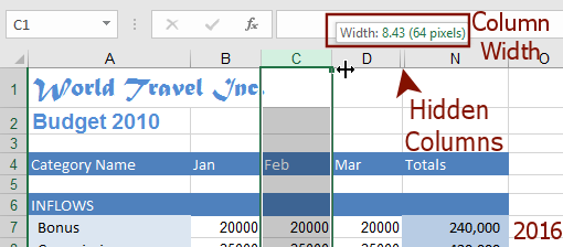
Column Width is measured in characters. A column's width can be from 0 to 255 characters, which is a REALLY wide column! Decimal values are allowed. In fact the default size is 8.43 characters (= 64 pixels where a pixel is the smallest dot on the screen).
A width of 12, for example, means the column is wide enough for 12 average characters, using the Body font for the current theme. The default for the blank document template is Calibri 11 pts. This changes if you set a specific font in the dialog Excel Options > General > Use this font, or if you use a different template to start your document.
![]() Hide column: A width of zero hides the column.
Or you can select one or more columns and use the Hide command in the right click menu or on
the menu for the Format Cells button. The column is
not deleted. It's just does not show.
Hide column: A width of zero hides the column.
Or you can select one or more columns and use the Hide command in the right click menu or on
the menu for the Format Cells button. The column is
not deleted. It's just does not show.
![]()
![]() Excel 2007, 2010: The only way to tell that columns are hidden is to read the column labels. Boo.
Excel 2007, 2010: The only way to tell that columns are hidden is to read the column labels. Boo.
![]()
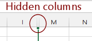
![]() Excel 2013, 2016: Shows a gap on the column headings (but not in the grid) when one or more columns are hidden. In the illustration, columns J, K, and L are hidden.
Excel 2013, 2016: Shows a gap on the column headings (but not in the grid) when one or more columns are hidden. In the illustration, columns J, K, and L are hidden.
![]() Unhide a hidden
column: Select the hidden column by dragging to select the visible columns on
either side. Use one of the methods below:
Unhide a hidden
column: Select the hidden column by dragging to select the visible columns on
either side. Use one of the methods below:
- Set the column width for all the selected columns to something besides zero
- Right click the selection and select Unhide from the context menu.
- Use the Unhide command on the menu for the Format Cells button.
| |
Step-by-Step: Format Columns |
|
| What you will learn: | to adjust column width with AutoFit for selection to adjust column width to widest item in column with AutoFit to adjust column width by dragging to adjust column width with dialog |
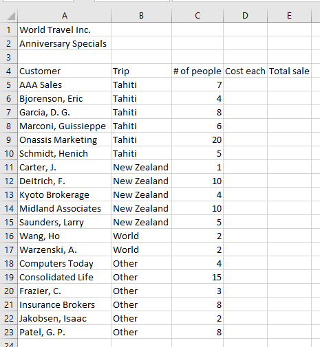
Start with: ![]() trips2-Lastname-Firstname.xlsx (saved in previous lesson)
trips2-Lastname-Firstname.xlsx (saved in previous lesson)
Column Width: AutoFit selection
You sometimes want a column to be wide enough for a particular cell's contents, but want other cells to wrap any longer lines in them. You will learn about the wrap command later.
 Save
As trips3-Lastname-Firstname.xlsx on
your Class disk in the folder excel project2.
Save
As trips3-Lastname-Firstname.xlsx on
your Class disk in the folder excel project2.
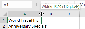
 Select cell A1, World Travel Inc.
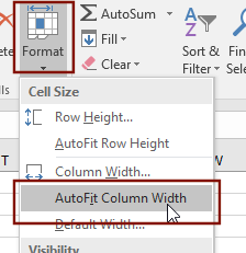
- On the Home tab in the Cells tab group, click on the button Format and then click on AutoFit Column Width.
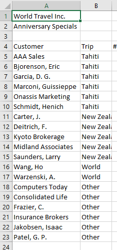
The column is resized just wide enough to hold the widest cell that is selected. In this case, there was only one, World Travel Inc.
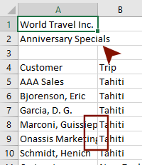 Note that cell A2 still overlaps its neighbor and several cells further down the sheet are cropped by the non-empty cells to the right.
If you had selected the column instead of just one cell, the column would widen
to fit the cell with the most text in it.
Note that cell A2 still overlaps its neighbor and several cells further down the sheet are cropped by the non-empty cells to the right.
If you had selected the column instead of just one cell, the column would widen
to fit the cell with the most text in it.
Column Width: AutoFit All
-
 Move your pointer to the right edge of the heading of Column A until it changes to
  the Resize Column shape.
 - Press the left mouse button down. (Don't release it yet.)
A screen tip appears, showing the current width of Column A in characters and in pixels.
- Release the left mouse button and double-click in the same spot (the right edge of Column A's heading).
The column width changes to display the longest text in any cell in the column as a single line. Wrap text: Sometimes you want text to wrap inside certain cells. For example a column of short numbers might have a label that is several words long, like Number of Customers . If you don't wrap such a label
inside the cell, there will be a lot of white space around the short numbers below it.
Wrap text: Sometimes you want text to wrap inside certain cells. For example a column of short numbers might have a label that is several words long, like Number of Customers . If you don't wrap such a label
inside the cell, there will be a lot of white space around the short numbers below it.  AutoFit surprises: The column may wind up wider than you expected. Any text will be on a single line in its cell. No matter how long the text is! If you accidentally find you've widened a cell out of sight to the right, use Undo. (Such a wonderful invention!) Then resize the column with another method.
Column Width: Drag
Dragging is a natural method of adjusting column width. But since you can't see the change until you release the mouse button, it may take you several attempts to get a satisfactory width.
-
 Move the pointer to the right edge of column heading B.
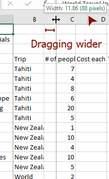
- When the pointer changes to the Resize Column shape, drag to the right until you think it is wide enough for New Zealand to show completely. (Yes, you must guess!)
 Confusing effect: As you drag, the column heading changes width, but the column itself does not resize until you release the mouse button. You may need several tries to get the width right. (The
screen tip in the illustration is a big hint!)
Confusing effect: As you drag, the column heading changes width, but the column itself does not resize until you release the mouse button. You may need several tries to get the width right. (The
screen tip in the illustration is a big hint!)
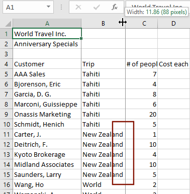 Click and hold again on the right edge of Column B to see the new width.
Column Width: Dialog
-
 Select a cell in Column C.
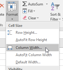
- On the Home tab in the Cells tab group, click on the Format button and then on Column Width.
The Column Width dialog appears.
-
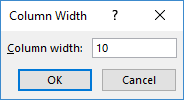 Type a new width of 10 and click OK.
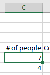
Now Column C is just large enough to hold the label # of People. There are 11 characters, including 2 spaces, in the column label. Spaces take less space in most fonts than other characters do. It takes some practice to make good guesses for widths measured in 'characters'.
 When you are having trouble dragging to get the width you need, use the dialog to set an exact width. This dialog is also good to use when you want several scattered columns to be the same width.
-
Save.
[trips3-Lastname-Firstname.xlsx]
|
|
| © 1997-2017 Jan Smith All Rights Reserved |
Site Map What's New |
Privacy Policy Terms of Service Copyright Acknowledgements |
~~ 1 Cor. 10:31 ...whatever you do, do it all for the glory of God. ~~
Last updated: March 22, 2017