
Jan's Working with Numbers
Design: WhatIf: Create
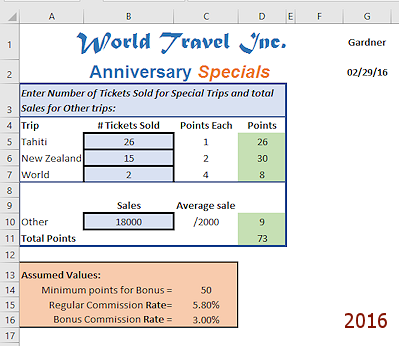
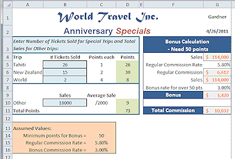
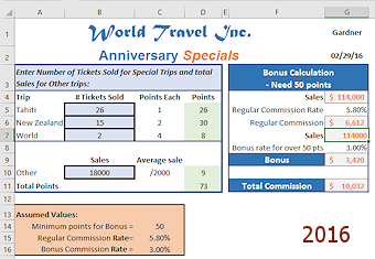
For the Anniversary Special Offers at World Travel Inc. there was a bonus for a travel agent based on points earned from his/her sales. You will create a What If spreadsheet for the travel agents to use to see whether they qualify yet for the bonus and how much the bonus would be.
Such a sheet would be helpful during the qualifying time period. An agent could use a Bonus Calculator to see if he had earned the bonus yet. If not, then he could play with the numbers to see what he needed to do to earn the bonus. A good motivation!
You will use the Planning Checklist and later you will document what you did.
Facts you need to know:
-
Tahiti trip = 1 point
-
New Zealand trip = 2 points
-
World trip = 4 points
-
Other trips = points are awarded by dividing the sales for Other trips by $2000, which is the estimated average cost of such trips.
-
Regular commission = 5.8% of sales.
-
Bonus = an additional 3% of sales, but only if the agent earns at least 50 points.
You must calculate an agent's number of points earned, the regular commission, the bonus commission, and the total commission.
Design Layout Considerations:
-
Will be used primarily on the screen rather than in print.
Everything an agent needs to see should fit on one screen at 800 x 600 resolution.
Agents often use small tablets or phones to work with the sheet. -
Data entry cells for the number of trips and sales amounts for Other trips should be obvious.
-
It should be easy to tell the calculated values (number of points and commissions) from the data entered and the fixed values (points each type of trip is worth, commission percentage, bonus percentage).
-
Results of calculations (Total Points, Bonus, and Total Commission) should stand out from the other areas.
Printing considerations:
The sheet should print on one page in portrait orientation. It should have include the agent's name and the date.
Plan of Attack
To help keep things organized, you are going to create three tables on the sheet-
-
Assumed values table: Fixed numbers used in the formulas
-
Entry table: Cells to enter sales info. Calculates and displays the points.
-
Results table: Calculates and displays the bonus and total commission
| |
Step-by-Step: Create a What If Sheet |
|
| What you will learn: | to plan a What-If sheet:
to create a table of assumed values to create a data entry table to create a results table to create a concatenated label |
Start with: ![]() trips32-Lastname-Firstname.xlsx(saved in previous lesson)
trips32-Lastname-Firstname.xlsx(saved in previous lesson)
Remember: To enter a value or a formula you must either press ENTER or click the ![]() check mark button after you've finished creating the contents.
check mark button after you've finished creating the contents.
Set Goals; Identify Inputs and Outputs
-
 From the facts stated above, on a separate sheet of paper complete the first two steps of the Planning Checklist for Spreadsheets.
[1. Set goals, 2. Identify Inputs and Outputs]Correct your work later if you find that you left something out. You will use this information to document the sheet in a Comment later.
Design Layout
- Draw a sketch of a possible layout design for your sheet. It
might be better than what you will be directed to do, which is shown at the
right. When you turn in your work to your teacher, attach the sketch of your layout.
The parts must be close together to meet the requirement that all fits on one screen at 800 x 600 resolution.
Sheet and Titles
You will create a new sheet for the Bonus Calculator. Remember that you have to copy the title cells to keep the formatting.
- Open trips32-Lastname-Firstname.xlsx , if necessary.
-
 Save As trips33-Lastname-Firstname.xlsx in the folder excel project5 on your
Class disk.
Save As trips33-Lastname-Firstname.xlsx in the folder excel project5 on your
Class disk. - Right click on the sheet tabs and select Insert… and from the dialog select Worksheet.
- Rename the sheet Bonus.
- Switch to the sheet Tahiti; select cells A1 and A2. Copy them.
Why copy from this sheet? On the sheet Specials, A1 has an attached comment that is not needed on the new sheet. - Switch to sheet Bonus, select cell A1, and Paste.
- Save.
[trips33-Lastname-Firstname.xlsx]
Customize
-
 In cell G1 type [Name] . The agent will replace this with his own name.
- In G2 type =TODAY()
After the word TODAY those symbols are an opening parenthesis and a closing parenthesis. Each time the sheet is opened, this function will display the system date, which is the date that the computer thinks it is. - Format by making both G1 and G2 bold and centered and vertically aligned Middle.
- Save.
[trips33-Lastname-Firstname.xlsx]
Table: Assumed Values
Using a table to hold the constant values used in your formulas makes it easy to change them later if the rules for the bonus change, perhaps for a different set of special offers. Once you have finished this sheet, you would be able to change the minimum number of points, for example, by changing the value in one place - this table.
 Enter Labels and Values: Starting with cell A13, enter the values as in the illustration.
The text lines below Assumed Values are in column B. They won't look like the illustration just yet.
- Format:
For the table title (cell A13), bold.
Center the values in cells C14, C15, and C16.Resize the title cell height by changing Row 13 to a height of 19.50 (26 pixels).
For the labels in column B (cells B14, B15, and B16), align right and widen column B to 16.43 (120 pixels), which is just enough to show the entire label and be indented a bit under the title in A13.
Select the whole table (range A13: C16) and fill with Orange, Accent 6 in Excel 2007 and 2010 or Accent 2 in Excel 2013 and 2016, Lighter 60% and border the whole table with a thick box border.
- Save.
[trips33-Lastname-Firstname.xlsx]
Table: Data Entry - Tickets and Sales
The next table is for the data an agent must enter about the number of trips. It will calculate how many points he has earned. You will fill in the table with data for Gardner.
The colors will be somewhat different in Excel 2013 and 2016.
-
 Enter Labels: Starting with cell A3 enter the labels as shown in the illustration for the table to
calculate points earned.
Enter Labels: Starting with cell A3 enter the labels as shown in the illustration for the table to
calculate points earned.
For cell C10, you must be in Edit mode or Excel will think this a formula and refuse to let you type the 2000.
- Format: Merge & Center A3:D3, wrap the text, left align, and vertical align as Middle.
Resize Row 3 to show all of the wrapped text.
Resize column A to show all of 'New Zealand' in the column.
Resize column C to show the entire label, 'Average sale'. Do not AutoFit column B. It would be far too wide because of the labels in rows 14, 15, and 16. - Formulas: Values in column D should be calculated by multiplying the value in column B for Tickets Sold by the Points each in column C. So the formula for D5 is =B5*C5 . Enter this formula and use AutoFill to copy it down to D6 and D7.
All the formulas result in a zero for now, since there are no values in column B yet.The points for Other trips in D10 are calculated by dividing the value in B10 by 2000. Enter the formula for D10 as =B10/2000 . The points will be rounded automatically in General number format.
The formula for Total Points is in cell D11 is the sum of all the points above.
Use AutoSum and modify the formula by dragging the selection area. -
 Enter Data: Change cell G1 to Gardner .
Switch to sheet Specials. Identify the trips that Gardner sold.
Add up the number of tickets Gardner sold for each trip and enter those numbers in sheet Bonus cells B5:B7.
Add up Gardner's total sales for the Other trips. Enter that number in cell B10 of sheet Bonus. - Format:
[Actual colors are somewhat different between versions. Illustrations are not all from the same version!]
To make the places for data entry obvious, border those cells with a thicker black line and fill those cells with Accent 5, Lighter 80%. (Cells B5, B6, B7, B10)
Use the same fill color but no border on the directions in cell A3. It's nice to coordinate your colors!Turn off the display of grid lines. [Ribbon tab View > uncheck box for Grid lines]
Now the borders and fill color clearly show where you are to type in data. (Working without the grid lines is possible with a small table, but it is not a easy as it sounds. Another experience for you!)Format the calculated values differently by filling those cells with pale green: In Excel 2007 and 2010 = Accent 3, Lighter 60%. In Excel 2013 and 2016, Accent 6, Lighter 60%.
(Cells D5, D6, D7, D10, D11) Make the column labels (Cells A4:D4 and B9 and C9) and the row
label Total Points in cell A11 bold. Make the directions in cell A3 bold and italics.
Make the column labels (Cells A4:D4 and B9 and C9) and the row
label Total Points in cell A11 bold. Make the directions in cell A3 bold and italics. Center all the columns of data and the calculations (B4:D11).
Resize columns if necessary to show the cell contents.
 Select the whole table,
including the directions.(A3:D11)
Select the whole table,
including the directions.(A3:D11)
Put a heavy border around the table in the color Accent 5, Darker 25%.Then select the directions and A7:D7 and add a heavy border in Accent 5, Darker 25% on the bottom edge of the selections.
-
Resize Row 3 to a height of 33.75 (45 pixels) and Column E to a width of 1.00 (12 pixels).
-
Save.
[trips33-Lastname-Firstname.xlsx]
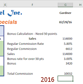
Table of Results: Commissions
This table will calculate the agent's regular commission and the bonus, and then will add them together for the total commission.
-
 Enter labels:
Starting in cell F3 enter the labels below for the table that will calculate commissions.
Bonus Calculation - Need 50 points
Sales
Regular Commission Rate
Regular Commission
Sales
Bonus rate for over 50 pts
Bonus
Total Commission(Watch cell F6 and F9. These may try to autocomplete with the text from the cell above, which is not right!)
Widen column F to show the whole text of cell F8, Bonus rate for over 50 pts.
Note: The new labels may get automatically formatted like the calculated cells to the left, even though there is a blank column in between. Surprise! You will work on the formatting later.
Problem: If you change the minimum number of points needed to get the bonus, your formulas that use cell C14 will automatically update but your labels in F3 and F8 will not be updated. You can fix that next with a formula that combines text and cell values!
- Save.
[trips33-Lastname-Firstname.xlsx] - Create label that will update by using a formula:
- Select cell F3 and type ="Bonus Calculation - Need " & C14 & " points"
- Quotes " go around the text and spaces you want.
- Replace the value 50 for the number of points with its cell reference C14.
- An & (ampersand) is needed to glue together text (in quotes) and a cell reference.
The action of combining different types of data with & is called concatenation.
By using this formula, if you change number of points in C14, the label changes automatically.
- Select cell F8 and edit this label so the number of points will also update automatically:
="Bonus Rate for over " & C14 & " pts"
 Problem:
Message says there is an error in the formula
Problem:
Message says there is an error in the formula
The message does NOT tell you what the error is!! Probably you left something out like one of the quotes or an & or mistyped the cell reference.
Solution: Proof-read your formula. Be sure you have matching sets of quotes and that there is an & between quoted text and any cell reference. - Select cell F3 and type ="Bonus Calculation - Need " & C14 & " points"
- Save.
[trips33-Lastname-Firstname.xlsx]
 Assumed Values: Link the cells for Regular Commission Rate and Bonus Rate to the Assumed Values table. You can
more easily see where to change these rates in the future if they are in a
separate table.
In most spreadsheets, good practices would put these fixed values on a separate
sheet where they can be easily found.
Assumed Values: Link the cells for Regular Commission Rate and Bonus Rate to the Assumed Values table. You can
more easily see where to change these rates in the future if they are in a
separate table.
In most spreadsheets, good practices would put these fixed values on a separate
sheet where they can be easily found.
For the Regular Commission Rate in cell G5 type = and click cell C15 in the table of Assumed Values and press ENTER.
For the Bonus Rate in cell G8, type = and click cell C16 in the table of Assumed Values and press ENTER.
- Save.
[trips33-Lastname-Firstname.xlsx]
- Formulas: The easy way to enter these formulas is to type the equals sign and the other symbols, but click on the cell to use.
Sales in cell G4 will require a longer formula than the others. Sales should be the sum of the sales for Tahiti, New Zealand, World, and Others. You already have the amount of the sales for Others in cell B10, but you must calculate that for the Tahiti, New Zealand, and World trips. You will multiply the number of tickets by the price per ticket. For example, the Tahiti sales will be the number of tickets times $1500 for each ticket, or =B5*1500. The cost of the trip is not on this sheet. It won't be changing either, so you can use the actual number this time instead of a cell reference.
 So your formula for G4 is =B5*1500+B6*3000+B7*6000+B10 .
Remember that all multiplications are done before the additions. If you like, you can add parentheses to make it clearer:
=(B5*1500)+(B6*3000)+(B7*6000)+B10)You calculate the Regular Commission by multiplying Sales by the Regular Commission Rate.
So in cell G6 you need = G4*G5Sales is repeated in G7 so you can see that you are going to multiply it by the Bonus Rate to get the Bonus.
So for G7 you just need =G4 .The Bonus in cell G9 is the Sales times the Bonus Rate, which is =G7*G8 .
The Total Commission in G11 is the sum of the Bonus and the Regular Commission, =G6+G9.
- Save.
[trips33-Lastname-Firstname.xlsx]
 Format: Apply the cell style Calculation to the calculated values in column G (cells G4, G6, G7,
G9, G11) and then apply Accounting style from the drop list. Reduce
decimals twice.
Format: Apply the cell style Calculation to the calculated values in column G (cells G4, G6, G7,
G9, G11) and then apply Accounting style from the drop list. Reduce
decimals twice.
Create a cell style named Label:
Fill Blue, Accent 1, Darker 25%
Font color: White;
Bold;
Font Size 12 pt.
Apply the new cell style to cells F3, F9, and F11.Use Merge and Center on the title to span F3 and G3. Turn on Text Wrap.
To make the title wrap nicely, we need to add a line break in the concatenated title.
Click in F3 to get into Edit mode so you can edit directly in the cell. Put the cursor at the end of 'Bonus Calculation'.
Use the key combo ALT + ENTER to put in a line break. The Formula bar will show only part of your formula because there is now a line break. Not to fear!
Press ENTER and the cell will show the label on two rows.Right justify F4: F8. Wide column F if necessary to get all the text inside the column.
Select the whole table (F3:G11) and apply a heavy border with the color Blue, Accent 1, Darker 25%
- Save.
[trips33-Lastname-Firstname.xlsx]
Bonus sheet created
|
|
| © 1997-2017 Jan Smith All Rights Reserved |
Site Map What's New |
Privacy Policy Terms of Service Copyright Acknowledgements |
~~ 1 Cor. 10:31 ...whatever you do, do it all for the glory of God. ~~
Last updated: March 22, 2017