Jan's Working with Numbers

Step-by-Step: Test Your Sheet

---

What you will learn:

to test fit to screen to test with easy numbers to test with special numbers to document the sheet to create a data validation input message to change the theme and see how it affects the sheet

---

Start with: trips33-Lastname-Firstname.xlsx(saved in previous lesson)

Test Fit to Screen

Monitors offer higher and higher resolutions these days, even on small screens like smart phones. If your monitor is using a resolution besides the one you are designing for, you cannot tell by looking at your screen if your layout will fit. You need to either change the resolution of your monitor, or resize the window to the resolution you want to check. Use one of the following to see how your sheet fits in the required 800 x 600 resolution:

• Switch resolution with your video card software: Some video cards allow you to switch the resolution of the monitor without having to reboot the computer. If yours does, you are in good shape! The choice is often in a popup menu from an icon in the Tray at the right of the Windows Taskbar. Otherwise, check out Display Properties (right click on the Desktop and choose Screen resolution or Properties > Settings tab). If you have to reboot to change to that resolution, use another method instead. It's not worth that effort.
• Switch resolution with other software: There are other programs that let you switch the monitor resolution, like the Power Toy QuickRes for older versions of Windows.
• Set browser size with software: Programs like Browser Sizer open a browser window for you that is a particular size, like 640 x 480 or 800 x 600. Very handy!
• Set browser size manually: Make an image that is the right size and resize your window the same size.

  Open Paint.
  Paint in WinXP and Vista:  Resize the blank default canvas to 800 pixels wide and 600 pixels tall using Image > Attributes. (Pixels are called pels in the dialog.)
  Paint in Win7 and later: Click the Resize button and uncheck the box "Maintain aspect ratio". Change the width to 800 pixels and the height to 600 pixels.

  
  Paint in Vista and Windows 7: Create a 800 x 600 image

  Fill the blank white canvas with a bright color. (The illustrations use Red.)
  Be sure that the whole rectangle is showing in the window. Resize the Paint window if necessary.

  Switch to Excel with the sheet you want to check as the active sheet at 100% Zoom. If necessary, maximize the sheet in Excel's window. Do not have Excel itself maximized.

  Position the upper left corner of Excel's window on top of the colored image in Paint. Drag the edges of Excel's window until the whole window is the size the Paint image. Ta Da! What you see is what you would see at 800 x 600 resolution with Excel maximized.

  You can gain more screen space for your spreadsheet by minimizing the ribbon. Right click on the ribbon and choose Minimize ribbon or Collapse ribbon.

  You can save your Paint image to use later if you need to do this kind of check often.
  

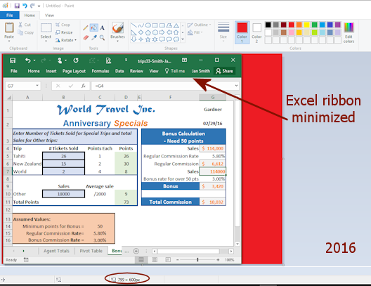
Excel window positioned over Paint image 800 x 600 pixels: 
With Excel ribbon minimized (Excel 2016)

If your sheet  winds up too wide for the screen, what could you do about it?
Some possibilities:

• Reduce the width of one or more columns
• Reduce the font size and then the width of one or more columns
• Rearrange your sheet

---

Test Calculations: Easy Numbers

Your formulas look like they are working while using this "realistic" data. But it's hard to be sure. It would be easy to have dropped a zero or to leave out a part of a formula or to have accidentally stuck in an extra cell reference while clicking around. You need to check your formulas with numbers that are easy to work with. In fact, it would make a lot of sense to start out with really easy numbers and then test with realistic data later.

Do not save with the data you enter for testing!!

1. Save as  trips34-Lastname-Firstname.xlsx  to the excel project5 folder on your Class disk.  
2. Before you continue, make a note of Gardner's numbers in column B. You will need to put them back in after testing is done.
   
3. Replace the Assumed Values:
   Use 10, 10%, 10%. Did the concatenated labels in F3 and F8 update?
   
4. Replace Data Values: Replace the # Tickets Sold with 10, 10, 10 and the Sales of Other trips with 10000.
   

5. Check Calculations: Check values in column D. Since you used numbers that are easy to calculate with in your head, you can easily see that the Points and Total Points are working well.

   Check the values in column G. Only the Sales in G4 is not obviously right or wrong. You did not include the cost of those trips on this sheet. Now we see a reason for doing it. Ah well. It will take just a little hand calculation to see if that is correct.
   

   • Tahiti = 10 tickets x $1500 = 15000
   • New Zealand = 10 tickets x $3000 = 30000
   • World = 10 tickets x $6000 = 60000
   • Other = 10000
   • Total = 15000 + 30000 + 60000 + 10000 = 115000. Correct!
     

---

Test Calculations: Special Numbers

Before you can say that your formulas are definitely working right, you must check out some special situations. What happens if some of the numbers are not there? Will the spacing be big enough for the largest and smallest numbers likely to be used? Test it out!

Do not save with the following changes!!!

1. Zeros: One at a time, replace each of the data numbers for Tickets Sold and the Assumed Values with a zero. (Do not forget to press ENTER or click the check mark button to actually enter the value.) Does the table still give good answers? Undo between each change.
   
2. Large/Small Numbers: Change the number of tickets sold for Tahiti to the largest number you think is likely to be sold. Are the cells for calculated values wide enough? If not, widen the column. Try some other large values in different parts of the sheet.

   At some point the Bonus and Total Commission will not fit in the column. The decision to make is which is more important- keeping the tables on one screen at 800 x 600 resolution, or having the cells wide enough to show really large sales? It's up to you.

   Are there formatting changes you could make to keep the tables on one screen and on one printed sheet and have still wider columns? So many choices!

   You should also test very small numbers, especially when negative numbers make sense on the sheet. This sheet would not use negative numbers, but the commission rate might be very small. What might be the smallest percentage likely to be used for the commission and bonus rates? How about small sale numbers? Try some to see if they are handled well by your formulas and cell sizes.

   Did you notice that the bonus is calculated even when the total points was too small to qualify for the bonus. That's a problem! You will handle that shortly.

3. Return the data to the values for Gardner.
   [Multiple Undo or close without saving and re-open]

---

Documentation

Your spreadsheet is designed, formatted, and tested. All that remains is to document what you did. Some documentation was done when you created titles and labels. Now you must create the Comments and Data Validation messages that will explain how the sheet works, who did it, etc.

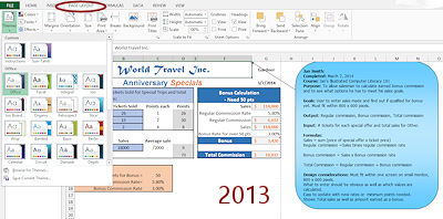
1. Main Comment: Select cell A1 and insert a Comment.
   Format the shape and color of the Comment's text box to suit yourself. Yes, you may be creative this time! Remember that to see the full dialog (and not just a Font tab) you must right click the comment's border.

   In this comment include -

   • your name
   • date completed
   • class for which it was done
   • Purpose
   • Planning Spreadsheets steps 1 and 2 from the previous lesson Create a What If Sheet.
     (Of course, your comments will not be exactly like the ones in the illustration.)
     • Goals
     • Output
     • Input
     • Formulas
     • Design Considerations
2. Other Comments: Select at least one cell containing a formula and create a comment that explains the formula in words.

---

Data Validation Message

1. Click B10. On the Data tab, click the button Data Validation and then on the tab for Input Message. 

2. For the Title, type Other Trips:

   For the Input message, enter On sheet Specials, select all of your Other trips. The Status bar will show the total. Enter that here.

   Click on OK.

   The message will appear whenever the cell is selected.

---

Finish

1. Page Setup: Open the Page Setup dialog to the Sheet tab and set Comments to At the end so that all comments will be printed on a separate page after the sheet prints.
2. Header: Create a header with your name and the date on the left, the file name and sheet name in the center, and Excel Project 5 on the right.
3. Spell Check. (This will check your comment text, too!)
   
4. Check the Print Preview. Comments should print on their own sheet. Data Validation messages do NOT appear in the list of comments.
5. Save as
    [trips34-Lastname-Firstname.xlsx]  
6. Print the Bonus sheet only. You should get 2 pages, the bonus calculator for Gardner and the comments at the end.

---

Change Theme

The colors you chose are from the current theme. What changes if you change the theme?
To see what is going on clearly with Live Preview, you may need to move the workbook out of the way of the Themes gallery.

1. On the Home ribbon tab, click the Dialog Launcher button for the Clipboard tab group.
   The Clipboard pane opens at the left of the window, which moves the table to the right.
2. Right click on A1 and select Show/Hide Comment to make the comment stay in view.
   (Your comment may not look like the illustration. You formatted it above to suit yourself!)
3. On the Page Layout tab, click on the Themes button to open the gallery of themes.
   With the Clipboard pane open, you can see all the parts as Live Preview changes them.
   
4. Hover over a few of the themes in the gallery.
   What parts of your sheet change?
          Font, Font size, Font color, Fill color
   What does not change?
         Comment features - none changed. Did you expect that?? The Format dialog does not use colors etc. from the theme!
         Calculation cell style: The font color and fill did not change but the font did.
   
5. On the Home tab, open the Cell Styles gallery and right click on the Calculation style.
   This style was applied to the calculated values in column G. (Make sure yours are using this style.)
   
6. Choose Modify Style... and click on the Format button.
7. Look on the Font tab at the Font box.
   It shows the Headings font from the current theme. That's why the font could change with a different theme.
   

8. On the Font tab in the dialog, click the Color button to open the palette of colors.
   None of these colors is selected. That means that the current color is not one on the theme palette. That's why it did not change when you hovered over a different theme.
   

   The Fill color behaves the same way as Font color, but a light gray works fine with all of the themes. You can leave that setting alone this time.
   

9. For the Font color, select the nearest color on the theme colors palette to the current color.
   
10. Click on OK to close the Format dialog and click on OK again to close the Style dialog.
    
11. Right click cell A1 and select Hide Comment
    

12. Hover over each theme.
    Now the calculated cells change font color. Is this helping or hurting??

    Which theme do you like best? Which is worst? (Remember that the list of themes is different for each version of Excel.)
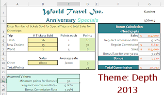
    Do all of the themes make it easy to see how this calculator works?
    Do you like a theme that uses shades of similar colors (Trek) or do you like wildly different, bright colors (Verve)? Or perhaps shades that are different but not vivid (Depth).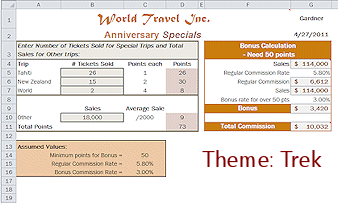

    

13. Click on the theme you like best to apply it.
    
14. Save trips34-mytheme-Lastname-Firstname.xlsx  to the excel project5 folder on your Class disk. 
    Your instructor may want you to print this or to submit it electronically.