Jan's Working with Numbers

Step-by-Step: Cell Styles

---

What you will learn:

to open an existing workbook to create a cell style   to apply a cell style to check what style a cell has   to modify a cell style to merge cell styles from another workbook to wrap text

---

Start with: trips12-Lastname-Firstname.xlsx  (saved in a previous lesson)

Open an Existing Workbook

There are many ways to open an existing file.

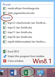
• Recent file list:
  • WinXP, Vista, Win7: Start menu > Recent Items
  • Win7, Win8, Win8.1, Win10: Excel Taskbar icon - Right click > Recent
    
  • Inside Excel:

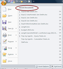
    Excel 2007: Office button menu > Recent Documents

    Excel 2010: File tab > Recent

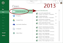
    Excel 2013, 2016: File tab > Open > Recent Excel 2016 groups recent workbooks by date.

• Computer/File Explorer window showing your Class disk, folder excel project3
  

1. Open   trips12-Lastname-Firstname.xlsx  from your Class disk.
2. Save as trips13-Lastname-Firstname.xlsx.  

---

Create a Cell Style

The first cell style you will create will duplicate the formatting in the header row, row 4. You could apply the same table style to the bottom section of data, but that pulls in a lot of features that are just not needed for such a small table. Besides, this lesson is on cell styles!

1. Select cell A4 =  Customer 
   This cell got its formatting from the table style Medium 2, but you converted the table back to a range.

   If you still see arrows in the row 4 cells, convert the table back to a range.
   Table Tools: Design > Convert to range button

2. On the Home tab in the Styles tab group, click the More button to show the gallery of cell styles.
   Styles are in groups: Good, Bad, and Neutral; Data and Mode; Titles and Headings; Number Format.

   When you create a custom style, it will show at the top in a new section, Custom.
   

3. Click on New Cell Style...

   The dialog shows the formatting for the current cell, A4, including what the table style added. The list of formatting is nicely detailed, except for Fill, which does not name the color. An odd omission!

   Problem: Dialog shows the default format
   The Font background, Border, and Fill settings are incorrect.
   You skipped a step and did not convert the table to a range.
   Solution: On the Data ribbon tab, click on Convert to Range and then on OK. Open the New Cell Style dialog again.
   
4. Type a new Style name in the box: Header Row
   

5. Click the Format... button.
   The Format Cells dialog appears, where you can view or modify all of the settings.

   You don't need to modify anything right now.

6. Click on each tab in this dialog and notice what the choices are and what the current choice is.

   By the way, on the Font tab, the Preview box looks like it has no sample text. The font color is White, so the text is there, as white text on a white background. Invisible!

7. Click the OK button to close the Format Cells dialog.
   

8. Click on OK again to close the Style dialog.
   The new style appears in the Styles gallery on the Home ribbon tab and is conveniently listed first.
    

---

Apply Cell Style

1. Select range A27:E27.

2. Click on the cell style Header Row in the gallery of cell styles.
   All of the labels for the second section of data are now formatted like the first table.

   
   Deleting a cell style: If you delete a cell style, any cells formatted with that style revert to the default style.

---

Which Style?

You cannot tell by looking whether or not a cell has a cell style applied to it. The Style gallery comes to the rescue!

1. Select cell E27.
2. Look at the Styles gallery on the Home tab.
   The style with the colored border is the current style, Header Row. Of course you might have to open the full palette to see the style.

---

Modify Cell Style

1. Right click on Header Row in the Styles gallery.
   A menu appears.
2. Click on Modify...
   The Style dialog appears.
3. Click on the button Format...
   The Format Cells dialog appears, open to the Font tab.
    
4. Change the Font to Cambria and the Font Size to 14.
   

    

5. Click on OK to close the Format Cells dialog.
   The Style dialog now shows the new Font settings.

   Live Preview does NOT show what effect this change will have.
    

6. Click on OK to close the Style dialog.
   The Style gallery shows the new formatting. All cells in row 27 to which you applied the Header Row cell style are using the new formatting. Sweet!

   What about the cells in row 4 from which we got the formatting?
   No, they stayed the same! You never applied the cell style to them.
   

7. Save.
   [trips13-Lastname-Firstname.xlsx]
   
    

---

Merge Cell Styles

Your new custom style is not seen by other workbooks. You can use the Merge Styles command at the bottom of the Styles menu to import styles from another workbook. Both workbooks must be open before you use that command. You can import styles even if they have the same name.

Did you think this command would merge two particular cell styles? I did!

1. Click the following link to download the workbook:
   styles-merge.xlsx

   This link opens the copy in the resources folder either from the online site or your local copy of the site. You can also go to where you saved the resource files if you wish.
   

2. Open this workbook in Excel.
3. Switch back to trips13-Firstname-Lastnme.xlsx and be sure that Sheet1 is the active sheet.
   
4. Click the More button for the Styles gallery.
   This gallery already has
   
5. Click on Merge Styles... at the bottom of the gallery.
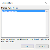
   The Merge Styles dialog opens.
   The dialog lists the other open workbooks.
   
6. Click on styles-merge.xlsx to select it.
   

7. Click on OK to close the dialog.
   The Styles gallery now shows two new styles in the Custom section, Dates and Totals.

   Notice that the custom cell styles are listed first, in alphabetical order.
   

8. Save.
   [trips13-Lastname-Firstname.xlsx]
   

---

Apply Cell Styles

1. Select B28:B35, the dates in the bottom table.
   
2. Click on the Dates cell style to apply it.
   
3. Select cells E25 and D37, the total sales.
   
4. Apply the Totals cell style.
   
5. Save.
   [trips13-Lastname-Firstname.xlsx]
    

---

Wrap Text

When your text is too long to fit in the cell's width, you can force the text to wrap inside the cell. This is often better than just widening the column enough for the text to fit.

1. Select cell C4.
   
2. Edit the text to read Number of people
   This replaces the existing text, # of people.
   
3. Similarly, replace the text in cell C27 with Number of people.
   In both C4 and C27 the text is cut off at the right.
   
4. Select C4 and C27 at the same time.
   (Hint: Hold CTRL down when you click the second cell.)
   
5. On the Home tab in the Alignment tab group, click on the button Wrap Text.
   Rows 4 and 27 immediately get taller to hold a second line of text. The text is still aligned Left.
   
6. Save.
   [trips13-Lastname-Firstname.xlsx]
7. Close the file styles-merge.xlsx