
Jan's Working with Numbers
Format: Cells: Modify Table
Excel thumbnails for table styles 

 show a header
row and four rows, which is just enough to show any alternating colors. You can also see whether borders are showing.
show a header
row and four rows, which is just enough to show any alternating colors. You can also see whether borders are showing.
Once you have defined a table, the Table Tools: Design tab lets you choose several other features for your table style to manage. You can mix and match these options and the style thumbnails will automatically update. Some table styles do not include formatting for all of the options.
You can rearrange your table by sorting on any column. Sorting multiple times in a sequence (carefully!) can work well or it might give very unhappy results, depending on your choices!
Applying a filter will hide rows that do not match your criteria. For example, in a table of customer orders, you could filter to see orders from a particular person or company. Or perhaps you are looking for a particular order that was for $152.95 but you cannot remember who placed the order. A filter on the order's total would hide all orders for other amounts. The orders are not removed from the spreadsheet. They are just hidden while the filter is in place.
The danger to filtering is, of course, forgetting that what you see is filtered!
| |
Step-by-Step: Modify Table |
|
| What you will learn: | to change a table's size to change table style options to sort and filter with table columns to filter on existing values to filter with a logical test to print a selection of a sheet to convert a table back to a range to clear all formatting |
Start with: ![]() trips11-Lastname-Firstname.xlsx (saved in previous lesson)
trips11-Lastname-Firstname.xlsx (saved in previous lesson)
- If necessary, open trips11-Lastname-Firstname.xlsx
 Save as trips12-Lastname-Firstname.xlsx in the excel project3 folder of your Class disk.
Change Table Size
You can modify several features of your table, like the size and whether or not there are special rows or columns.
The bottom
right cell of a table has a symbol in its bottom right corner. ![]()
When you hover over this corner symbol the mouse pointer changes to the
diagonal resize shape ![]() .
You can drag to increase or reduce the cells that are included in the table. Table
style formatting will change as you drag the table larger or
smaller.
.
You can drag to increase or reduce the cells that are included in the table. Table
style formatting will change as you drag the table larger or
smaller.
 Experiment: Change Table Size
- Click out of the table so you can see the corner symbol.
 Drag the bottom right corner of the table up a few rows and release
the mouse.
Drag the bottom right corner of the table up a few rows and release
the mouse.
The alternating colors vanish for the rows that are no longer in the 'table'.- Drag the bottom right corner back down.
 Drag left and then click out to deselect the table.
Only the cells that are currently in the 'table' are formatted with the table style.- Can you drag up and left at the same time? Down and right?
- When you are ready to continue... return the table to include
A4:E25.
If you get a warning about a circular reference, use Undo to return your table to its original state.
Change Table Style Options
 Click in the table somewhere.
The tab Table Tools: Design appears again.
The tab group Table Style Options has check boxes for special types of rows and columns. A table style might not include special formatting for some of these special table parts.The default table styles show a Header Row and Banded Rows, so those boxes are already checked.
The thumbnail cannot show that a column will be Bold or what font will be used.
-
 On
the tab Table Tools: Design in the Table Style Options tab group, click the box beside First Column.
On
the tab Table Tools: Design in the Table Style Options tab group, click the box beside First Column. What changed?
The first column of the table became bold.The thumbnail you saw did not show this.
 Click on Last Column and Banded Columns.
The last column turns bold. Alternate columns have colored fill now, just like the rows did. The effect can be rather odd, depending on the widths of the columns involved.
 Click on the box by Total Row.
This is not a change in formatting! A new row appears at the bottom of your table, just outside the table border.This works well ONLY when you did not already have a totals row!! Look at the value in row 26. It is double the lovely sum you already had in row 25. Clearly the total in the new row is adding up everything in the last column, including the total that was already there. Bad idea for this table!!
This new total row creates only a total for the last column. If you want other totals, you can create them on this row.
 Use
the Total Row option when you do not already have a totals row for
the table. This is especially useful when you want to look at how
some totals change as you filter the table temporarily.
Use
the Total Row option when you do not already have a totals row for
the table. This is especially useful when you want to look at how
some totals change as you filter the table temporarily.- Experiment: Special Rows and Columns
Try out several combinations of the choices in Table Style Options and various table styles.
Which do you think would work well with this particular table?When you are ready to continue...
Uncheck the boxes for Total Row, First Column, Last Column, and Banded Columns.
You should be back to the formatting you started with.It is not necessary to save since no changes were kept.
Sort Table
A 'table' in Excel can be sorted using a menu from the arrow in the column label. You hid those arrows in an earlier lesson.
The header row (row 4) gained a drop list for each column. Each arrow opens a menu of choices for sorting and filtering the whole table based on what's in that column. Sorting rearranges the rows. Filtering hides the rows that do not match the criteria that you pick.
- On the Data ribbon tab, with a table cell selected, click on the Filter button.
The down arrows reappear on the table's column headings.  Click outside the table to deselect the
table.
Click outside the table to deselect the
table.The column arrows did not disappear! This is one of the benefits of setting up cells as a table. You do not have to select the table again to use the commands on the arrow menu.
- Click the arrow for the first column to drop its menu.
You have several sorting choices and filtering choices.
-
 Select Sort A to Z.
What changed?
- Rows moved into alphabetical order by Customer name.
- Arrow button:
 has an up arrow.
 - Table formatting: Did not move with the
data. That's a good thing!
-
Original Totals row: Sorted with other rows. The calculated values changed! This could be a problem!
There is a green triangle in the corner that show that Excel thinks there IS a problem.
-
 Click in the cell with with green triangle and then click on the
error icon to see the message. "Inconsistent Formula". Look at the Formula bar. It shows =SUM(E2:E21)
Click in the cell with with green triangle and then click on the
error icon to see the message. "Inconsistent Formula". Look at the Formula bar. It shows =SUM(E2:E21)
but the last customer row is row 24. Moving the formula is making a mess!Total rows don't belong inside a table!
Leave your own totals row out of the 'table'. Then it won't be sorted!
-
 Open the Customer column list again and select Sort Z to A.
What changed?
- Rows moved into reverse alphabetical order by Customer name.
- Arrow button:
 has a down arrow.
 - Totals row: Moved again and got new values. Wow! Quite a change! The formula is adding up only the cells above it.
- Table formatting: Stays in place. Did not move with the row.
Undo twice!
Your table should be back the way it was before sorting, with the custom sort by trip with Tahiti first.Sorting formula cells: Do not
include a cell with a formula when sorting unless ALL relative cell references
in the formula are to cells in the same row.- Experiment: Sort
- Sort using other columns. Exactly what choices you see in the menu depends on the kind of data in the column.
Click on Sort by Color.
You will see choices here only when you have applied colored fill in cells with Cell Styles (which we will look at in a later lesson). The background fills from the table's style do not count. The Sort by Color choice also includes a link to the Sort dialog where you can sort on multiple columns, as you did in an earlier lesson.
When you are ready to continue...
- Undo all of your
experimentation. You should be back to how the table was
formatted at the beginning of this topic.
Filter Table: Match Existing Values
The choices in the Filter section of the menu depend on whether the data in the column is text or numbers. Once of the most common filters looks for one or more values that are known to be in the column. Those values show in the menu from the column's arrow.
-
 Click the arrow for the Trip column to open its list.
- Click the (Select All) box to deselect all values at once.
- Click on New Zealand and World.
-
 Click on OK to apply the filter you just created.
What changed?
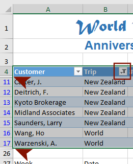
- Rows do not move but are hidden.
Look at the row headings. Numbers are missing! Only rows with a Trip value of New Zealand or World are visible. - Arrow button:
 gained a funnel, which is the symbol for a filter.
 - Totals row: Vanished.
- Table formatting: Applied to the visible
rows. Does not follow the data rows.
- Rows do not move but are hidden.
-
 Click the filter button on the Trip column again.
- Click Clear Filter
From "Trip".
The full table reappears. - Experiment: Filter
Try out filters on different columns and clear them.
What happens when you filter two different columns without clearing the first filter? - Use Undo multiple times to return the data to the original
arrangement - Sorted on the Trip column with a custom list, with
Tahiti first.
Filter Table: Logical Test
Sometime you want to see the rows where the values are less than a particular number, or greater than a certain value. Or you might want to search for values that start with a particular text.
-
 Click the arrow on the column Total sale.
The Sort and Filter menu appears. - Hover over Number
Filters to expand its submenu.
If the column contains text, you would see Text Filters instead.
 Click on Greater Than Or Equal To...
The Custom AutoFilter dialog opens, with the first text box already filled in with a logical test: is greater than or equal to.- Click the arrow in the text box at the top right.
A list of values in the column appears. - Click on 15000.
When 'And' is selected, both criteria must be met.
When 'Or' is selected, only one must be true, but it is OK if both are true. -
 Click the arrow beside the the second logical test and
scroll the list to see all of the possibilities.
Click the arrow beside the the second logical test and
scroll the list to see all of the possibilities.
Do not choose any of these at this time.
-
 Click on OK to close the dialog and apply your filter.
Only 5 rows of data and the Totals row still show. They are the only ones with a Total sale value of 15,000 or greater.The value in row 25 for Totals is not changed. It is still the total of all values, including the hidden ones.
- Experiment: Custom Filter
Try out other choices for a custom filter.
What happens when you combine filters with AND selected in the dialog?
What happens when you combine filters with OR selected?When you are ready to continue...
- Clear the filter.
Your table is back to its original status.
Print Selection
You can print just part of a spreadsheet by setting the Print Area, but that is permanent until you change the print area. For a temporary situation, it's better to select what you want to print and use the Print choices to print only that selection.
- Select the range A1:E25.
This is the upper table and the title and subtitle. - Open Print Preview and choose Print Selection:
 Excel 2007: Click the Office button and Print. In the Print dialog, click the radio
button for Print Selection, then click on Print Preview.
Excel 2007: Click the Office button and Print. In the Print dialog, click the radio
button for Print Selection, then click on Print Preview.

 Excel 2010, 2013, 2016: Open Print Preview. Change the settings, if necessary, to Print
Selection.
Excel 2010, 2013, 2016: Open Print Preview. Change the settings, if necessary, to Print
Selection.
- Verify that only A1:E25
will print!
Notice that the column arrows do not print! Yeah!! - If necessary, change orientation to Portrait.
 Print.
- Save.
[trips12-Lastname-Firstname.xlsx]
Convert Table to Range
Are you annoyed by those arrow buttons on each column? Once you get your table sorted, you can return the cells to an ordinary range, but the formatting and the sort order stay in place. Filters will be cleared automatically when you convert the table back to a range.
This is a fast way to remove all the cell formats and get back to basics - Normal font, no borders, no fills, no merged cells. To return to a previous stage in your formatting, you can use Undo. But Undo only remembers 100 actions. That sounds like a lot, but you can easily exceed that number in a single editing session!
-
 Switch back to Normal view and open the Name Box list.
Click on Table1.
Your list will show a different number if you created a table more than once during your work. The whole table
appears to be selected, but the header
row is outside the border. It is hard to see highlighting when the table color is similar to the highlight color!
The whole table
appears to be selected, but the header
row is outside the border. It is hard to see highlighting when the table color is similar to the highlight color!
-
 On
the Table Tools: Design tab in the Tools tab group, click on the Convert to Range button
On
the Table Tools: Design tab in the Tools tab group, click on the Convert to Range button 
 .
.
A message box asks if you want to convert the table to a normal range. - Click on Yes.
The columns arrows are gone but the table style formatting and sorting order remains. Any filters would be removed automatically.
Now that we are finished with table styles, let's get our formatting back on those amounts of money. -
 Apply Accounting style to E5:E23 and E25, with no decimal
places.
Apply Accounting style to E5:E23 and E25, with no decimal
places. - Save.
[trips12-Lastname-Firstname.xlsx]
Clear All Formats
One of the common uses for tables is to apply a table style for formatting. But suppose you need to get rid of that formatting later? You can clear the formatting in several ways.
- In
the Name Box, type A1:E25 and press ENTER.
This selects all of the cells that you have been working with lately.
-
 From the Home tab in the Editing tab group, click the Clear button and then Clear
Formats.
From the Home tab in the Editing tab group, click the Clear button and then Clear
Formats.
All formatting is removed from the selection... except for the word 'Specials'. Unexpected! Because the formatting was not applied to the whole cell, it is not removed by Clear Formats. You could manually change each format or else delete the word and retype it - which is easier! - Save as trips12-clearformats-Lastname-Firstname.xlsx to the excel project3 folder on your Class disk.
-
 Open Print Preview.
 Problem:
Preview does not show all of the data
Problem:
Preview does not show all of the data
What happened?? Your print settings are still set to Print Selection.
Solution: Change the setting for the printer to Print Active Sheets.
- Print.
- Close the spreadsheet.
|
|
| © 1997-2017 Jan Smith All Rights Reserved |
Site Map What's New |
Privacy Policy Terms of Service Copyright Acknowledgements |
~~ 1 Cor. 10:31 ...whatever you do, do it all for the glory of God. ~~
Last updated: March 22, 2017