
Jan's Working with Numbers
Intro: Exercise Excel 1-2
 You
will format an existing sheet. You will make the
totals and labels stand out from the data.
You
will format an existing sheet. You will make the
totals and labels stand out from the data.
Exercise Excel 1-2: Half-Year Budget
| What you will do: | Save a copy of a spreadsheet Use AutoSum Sort rows Format numbers Save and print |
Start with:![]() , halfyear.xls from resource files
, halfyear.xls from resource files
Use the buttons for AutoSum and sorting to create totals and arrange the rows.
Save Copy of Spreadsheet
- From your resource files in the numbers
resources folder open the file halfyear.xls, or download the file directly.
This file contains some of the data from the budget-2010.xlsx worksheet that you have been working with, but it is formatted differently.
 Use Save As to save the workbook as ex1-2-Lastname-Firstname.xlsx to the excel project1 folder as a current Excel
worksheet, with type .xlsx, on your Class disk, using
your own first name and last name.
Use Save As to save the workbook as ex1-2-Lastname-Firstname.xlsx to the excel project1 folder as a current Excel
worksheet, with type .xlsx, on your Class disk, using
your own first name and last name.
AutoSum and Sort
![]() Tip: Have a blank cell between the cell with the Sum and the cells that are being added up. That makes it easier to add new rows or columns without messing up the formula.
Tip: Have a blank cell between the cell with the Sum and the cells that are being added up. That makes it easier to add new rows or columns without messing up the formula.
- Row Totals: Use AutoSum to create row totals in Column I. The formula will include the blank cell in column H. After you get two values in Column I, Excel will try to sum the column instead of the row. Change the range when that happens. Include the cell column H in your selection. Remember to press
ENTER to accept the formula.
- Sort: Sort the category rows, Rows 7 - 19, into alphabetical order.
Your formulas refer only to cells in the same row, so you will not mess up the formulas by sorting. Whew!
- Column Totals: Use AutoSum to create column totals in Row 21.
Again Excel will get confused after you have two values in the row. It will try to sum the row instead of the column. Change the range when that happens.
- Grand Total: In cell I22 use AutoSum to create a grand total, but change the range to include all the cells with Light Turquoise background, B7:H20. Type Grand Total = in cell G22.
Format Numbers
- Format currency: Format the new totals in column I and in Row 21 and cell I22 as Currency.
- Format decimals: With the cells still selected, click the button Decrease Decimal twice. Now no digits to the right of the decimal point are showing. Only one cell had anything but zeroes to the right. For cell I10 click the button Increase Decimal twice to show its full value.
- Format Painter: Use the Format Painter button to copy the format of cell
E14 to range G22:I22, the grand total and its label. While that range is selected, make the cells bold. Reset I22 to Currency. Be sure that two decimal places show to the right.
-
 Header: Switch to Page Layout view and create a header. Type your name and
a space. Type the date and press ENTER to get a new line. Type Exercise Excel
1-2
Header: Switch to Page Layout view and create a header. Type your name and
a space. Type the date and press ENTER to get a new line. Type Exercise Excel
1-2
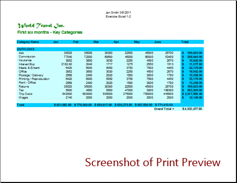
- Prepare to Print: Switch to Print Preview. Check what will print.
Make corrections if necessary.
- Change the page orientation to Landscape.
- Save.
[ex1-2-Lastname-Firstname.xlsx]
 Print.
-
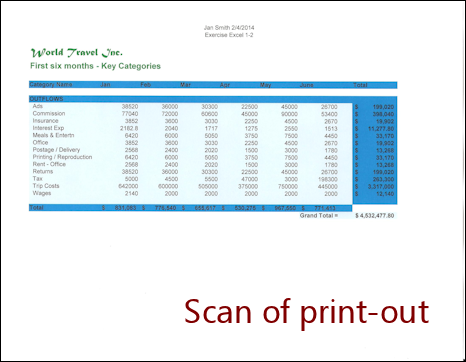 Evaluate: Are the colors on paper the same as you see on the screen?
Did these formatting choices work well on the printed page?
Many printers will print the dark blue as a darker color than you see on the screen.
Was black a good choice for the numbers and text on that dark blue background?
This worksheet is used in the next exercise.
|
|
| © 1997-2017 Jan Smith All Rights Reserved |
Site Map What's New |
Privacy Policy Terms of Service Copyright Acknowledgements |
~~ 1 Cor. 10:31 ...whatever you do, do it all for the glory of God. ~~
Last updated: March 27, 2017
These exercises use files from the numbers resource files. The default location for these files is c:\My Documents\complit101\numbers\ You cannot make changes to these files and save them in the same place. Save the changed documents to your Class disk. This keeps the original resource files intact in case you need to start over or another student will be using this same computer.