Jan's Working with Numbers

Step-by-Step: AutoSum

---

What you will learn:

to use AutoSum to total a column to use AutoSum to total a row to change range references in a formula

---

Start with: budget-2010-Lastname-Firstname.xlsx at Budget sheet from previous lesson

You will not be saving any changes in this lesson but your instructor may want you to capture some screen shots to prove you did the lesson. Ask.

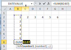
AutoSum: Column

1. If necessary, open budget-2010-Lastname-Firstname.xlsx.
   Verify that the active tab is Budget.
   
2. Select the cell B14, which is blank except for the colored fill. We will pretend that this is a good place for some new totals.
   
3. On the Home tab, click the AutoSum button .

   Excel guesses that you want to add the numbers above the selected cell up to the next blank cell, B6. It surrounds the range B7:B13 with a blinking dashed border. 

   The formula is displayed both in the Formula bar and in the cell. It will overlap other cells if necessary while you are working. 

   All formulas must begin with =, the equals sign.

   Cells added to formula by clicking: While the blinking dashed border surrounds the cells, clicking or dragging will change the formula, using the cell references of the cells you clicked or dragged. It can really foul up your calculations to click without careful thought. Pressing ESC will remove this blinking border and cancel your actions if you need to start over.
   

4. Press ENTER.
   The calculated value, 680500, is displayed now in cell B14 instead of the formula. The cell below (B15) is selected instead of B14.
    
   Default behavior: The selection moves down one cell when you press the ENTER key to register data in a cell.
    
5. Press the Up arrow on the keyboard.
   The selection moves up to B14. The formula shows in the Formula Bar but the calculated value still shows in the cell itself.
    

---

AutoSum: Drag to Change Range

If Excel guesses incorrectly, you can change the cell references.

1. With cell B14 selected, click the AutoSum button .
   Range B7:B13 is Excel's guess again about what you want to add up. Let's suppose we only want to add up cells B10 through B13.
   
2. While the blinking border is active, drag from B10 to B13 and release the mouse button.
   The cell references in the formula change. The total changes.

   Notice the screen tip that shows while you are dragging. It says that you have selected a region that is 4 rows high and 1 column wide.
   

3. Press ESC to cancel the AutoSum action without accepting the formula. 
   
4. Press DELETE to leave cell B14 blank again.
   

---

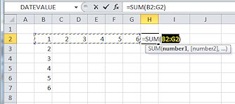
AutoSum: Row

AutoSum works for rows also.

1. Select cell N7.
   In the cell you see a number, but in the Formula Bar you see the formula that was used to calculate the number,  =SUM(B7:M7).
   
2. Press DELETE to remove this formula.
   
3. Click the AutoSum button.
   Excel guesses that you want to add the values in the cells to the left, with range reference B7:M7.
   You may have to use the horizontal scroll bar to see how far to the left the blinking border extends.
   
4. Click the check mark on the Formula bar.
   The sum is entered, but cell N7 remains selected.
   If you had pressed ENTER, the selection would have moved to the cell below.

---

AutoSum: Type to Change Range

1. With cell N7 selected, click in the Formula Bar.
   You can now change the formula yourself.
   
2. Edit the formula to read  =SUM(B7:M7,C9:J9, D11:L12)
   Be careful about the commas and colons in the formula.
   There is no logical reason to add these cells together, but we are only practicing.
   
3. Click the check mark button at the left of the Formula Bar.
   Your formula is accepted and the selection remains in cell N7.
   
4. Click in the Formula bar again.
   Suddenly there are colors in the formula! The matching cells or ranges gained the same color outline. Excel 2013 and 2016 also have a paler version of the color as a background color for the ranges in the formula.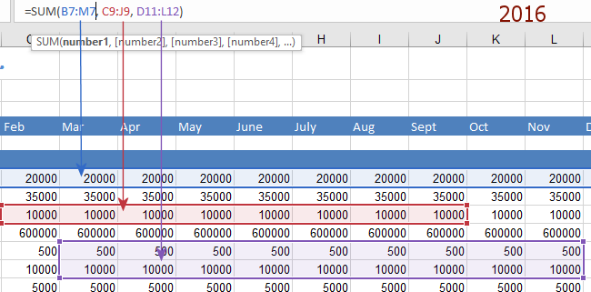

   

   Range finder:  Each range in the formula has a different color. A matching color surrounds the cells themselves. This can really help you see what is happening.

   Edit formula to see colors: Only when you are editing the formula will you see these colored references with matching borders and backgrounds.
   

5. Press ENTER to accept this odd formula.
   The calculated value shows in the cell and your selection moves down one cell.

   Cell N7 gained a green triangle in the upper left corner. This means that there are cells with numbers in them that are next to the cells in the formula. Excel is letting you know in case you missed some cells that you meant to catch with the formula.
   

6. Click on the Undo button repeatedly until the formula is back to the original, =SUM(B7:M7)
   
7. If you need to stop for now, close the spreadsheet but do not save changes.