Jan's Working with Numbers
Intro: Common Tasks: Format Numbers
Numbers can be written in different ways and still mean the same amount. For example, 1 can also be written as 1.00, 1.000, or 100%, depending on exactly what you are doing and how you want to look at your numbers.
[For the perfectionists out there: Yes, I know that there are differences in the exact meaning of the numbers above, especially for measurements. For most purposes in spreadsheets we can treat them as the same.]
 Excel includes
buttons on the ribbon for some of the most common ways to format numbers. Later you will use a dialog
that has even more choices.
![]() or
or  Accounting: (previously named Currency)
Formats the number as money, like showing the number 1 as $1.00
when your system is
set to use dollars. Excel comes in different languages, and will use the
appropriate local currency and decimal symbol based on the location in
Windows' Region & Language (on the Control Panel). The button may even change to
the general currency symbol! You are
not stuck with the default! The Currency button has a drop list of common
currencies and a command to open a longer list.
![]() Warning:
If you play around with the Region and Language settings, an open worksheet may
remember changes even after you return the settings to the originals!
Warning:
If you play around with the Region and Language settings, an open worksheet may
remember changes even after you return the settings to the originals!
![]() Percent: Formats the number as a percentage, like 100%.
Numbers are rounded by default so that 0.256 becomes 26% instead of 25.6%.
Percent: Formats the number as a percentage, like 100%.
Numbers are rounded by default so that 0.256 becomes 26% instead of 25.6%.
![]() Comma: Formats the number to show 2 digits to the
right of the decimal and separates every 3 digits to the left of the decimal. If
the location is United States, a comma is the symbol for the separator and a
period is the decimal. Other locations and other languages may reverse these symbols, using a period to separate and a comma as the
decimal symbol.
(Why doesn't the whole world do things the way I do?!)
Comma: Formats the number to show 2 digits to the
right of the decimal and separates every 3 digits to the left of the decimal. If
the location is United States, a comma is the symbol for the separator and a
period is the decimal. Other locations and other languages may reverse these symbols, using a period to separate and a comma as the
decimal symbol.
(Why doesn't the whole world do things the way I do?!)
![]() Increase/Decrease Decimals: Changes the number of
digits showing to the right
of the decimal. The number is rounded when decreasing decimals. When
increasing decimals, the original digits are shown, rounded to the number of
decimal places you have chosen. Excel remembers the actual number that was entered, no
matter how many digits you tell it to show.
Increase/Decrease Decimals: Changes the number of
digits showing to the right
of the decimal. The number is rounded when decreasing decimals. When
increasing decimals, the original digits are shown, rounded to the number of
decimal places you have chosen. Excel remembers the actual number that was entered, no
matter how many digits you tell it to show.
 Apparent errors in
calculated values:
Calculations use the underlying numbers in the cells, not the numbers that you see. This can make a difference in the results of the calculation.
Example: Adding the values displayed did not equal the calculated sum
Cell B2 = 512.46 and cell C2 = 66.6666. Cell D2 = B2 + C2, which is 579.1266.
Format the cells to show only one decimal point.
The cells B2 & C2 show the rounded values, but in D2, Excel first adds the original values and then rounds the answer. This is not the same as adding the rounded values that would add up to 579.2!


[Note to teachers: You may need to review percentages and rounding procedures with your students to be sure they understand both of these. VERY important when working with spreadsheets.]
| |
Step-by-Step: Number Formats |
|
| What you will learn: | to change number formats what each number format button does to use Format Painter to copy formatting |
Start with: ![]() budget-2010-chart-Lastname-Firstname.xlsx from previous lesson
budget-2010-chart-Lastname-Firstname.xlsx from previous lesson
Number Formats: Currency
 Save
As with the name budget-2010-formats-Lastname-Firstname.xlsx.
Save
As with the name budget-2010-formats-Lastname-Firstname.xlsx.-
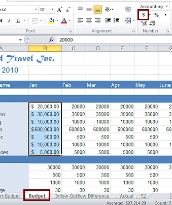 If
necessary, click the tab for the Budget sheet to make it the active sheet.
 - Select cells B7:B13.
- On the Home tab click
 the Currency button to apply the currency number format.
Now your numbers look like dollars, if that is the default currency on your computer. In another project you will learn how to change the currency being used.What changed:
- Added $ to the far left edge of the cell
- Added a decimal at the right of the whole numbers
- Shows exactly 2 digits to the right of the decimal
(Since the numbers were whole numbers to start with, this format adds 2 zeros.) - Commas divide groups of three digits to the left of the decimal.
- Column widened automatically to show all the digits and the $.
Number Formats: Percent
-
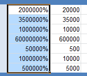 While B7:B13 is still selected, click
  the Percent button.
All the numbers are changed to percentages. Since these were large numbers, they look even larger as percentages.
What changed:
- Removed $ and commas.
- Added % at the right.
- Moved the two digits that were at the right of the decimal to the left.
Number Formats: Comma
-
 While B7:B13 is still selected, click
  the Comma button.
What changed:
- Removed %.
- Added commas to separate groups of 3 digits to the left of decimal.
- Shows 2 digits to the right of the decimal.
Number Formats: Change Decimals
-
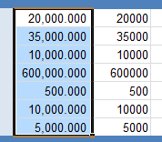 While B7:B13 is still selected, click
  the Increase Decimals button.
What changed:
- Gained another digit to the right of the decimal.
- The column automatically widened to show the new digits.
-
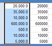 Click
Click  the Decrease Decimals button twice.
What changed:
- Only one zero is left to the right of the decimal.
- (The column width did not reduce its width.)
Copy Formatting: Format Painter
Excel and other Office programs have a handy tool for copying formatting from place to place, Format Painter.
-
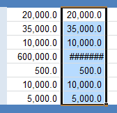 With
the previous formatting still selected, on the Home tab, click on the Format Painter button
  .
.
The mouse pointer changes to the Format Painter shape and the selected range gets a dashed border than moves like 'chase' lights.
Drag from C7 to C13.
The same comma formatting with only one decimal place is applied. The pointer returned to the usual shape and the Format Painter button is not colored anymore. But the column did not widen automatically like it did with the number format buttons.
Your sheet may show more cells with ######## than the illustration. What does ###### mean? The hash symbols, ########, mean that the column is
not wide enough to show the number. We won't worry with that at this
point. If you have used Zoom to reduce or enlarge the view, you
may see these ##### symbols in more cells. The number may still print fine. It depends!
 Always
check the Print Preview carefully to be sure all of the numbers will
print.
 -
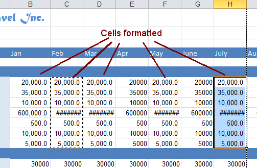 With
the C7:C13 still selected, double-click the Format Painter button
  .
.
Now the pointer will stay in Format Painter shape until you press the ESC key or else click the Format Painter button again.
- Drag across the ranges D7:D13, F7:F13, and H7:H13.
All these cells get the copied formatting without having to click on the Format Painter button again.
- Press the ESC key.
The mouse pointer returns to its normal shape and the Format Painter button loses its color.
 Save.
Save.
[budget-2010-formats-Lastname-Firstname.xlsx]
