 |
If you have worked with Windows
programs before, you already know a lot about Excel's window. It has all the
normal window parts, like the status bar, title bar, scroll bars, menu bar. The
Excel window is actually a lot like what you saw in Word. If you are
not familiar with Word, you should consider working at least the first
project of Working with
Words before continuing.
[This page is translated to Serbo-Croatian language at WebHostingGeeks.com]
What's Old, What's New
Click the image below of the Excel window to see what
parts of the interface are different from MS Word.
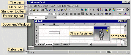
Click the image to see what's different
Illustrated with Excel 97, but all versions are similar
|
 |

Where you are:
JegsWorks >
Lessons >
Numbers
Before
you start...
Project 1: Excel Intro
Interface

Toolbars
Task
Pane
 
Smart Tags
 
 Open Excel Open Excel
Select & Navigate
Common Tasks
Summary
Quiz
Exercises
Project 2: Excel Basics
Project 3: Format & Arrange
Project
4: Groups & Formulas
Project 5: Design
Search
Glossary
Appendix
|
|
The Excel Window
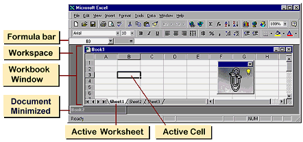
By default, newer versions of Excel put each Excel
spreadsheet into its own window. This behavior can be changed from the
menu Tools | Options | View tab - Show: uncheck the box for Windows in
Taskbar.
Terms
|
spreadsheet |
Document that is entirely made up of rows and columns. Used to list
and analyze data.
 Point of Confusion:
People tend to use the word
spreadsheet in two ways: Point of Confusion:
People tend to use the word
spreadsheet in two ways:
- the entire Excel workbook file
- an individual worksheet
|
| workbook |
The basic document for Excel.
Its filename uses the extension xls, from Excel spreadsheet. A workbook
usually contains several worksheets.
|
| worksheet |
A single sheet of data. One or more worksheets make a workbook.
Think of them as pieces of paper that are stacked on top of each other to
form the workbook.
The maximum number of
worksheets in a workbook depends on your computer's memory. The default
workbook can have up to 255 worksheets.
A worksheet, also called just a sheet
or spreadsheet, can have up to 256
columns and 65,536 rows with up to
32,000 characters in a single cell. This is enough for most purposes!
 But
it does mean that you can't easily use Excel to write a novel. But
it does mean that you can't easily use Excel to write a novel.
|
| workbook window |
The document window in an Excel window.
|
| cell |
Intersection of a row
and a column on a worksheet
|
| sheet tab |
Each worksheet has a tab at the bottom of the workbook window with the name of the worksheet on it.

|
| active worksheet |
The worksheet that receives your keystrokes and commands. It has a white tab and its name is bold.
|
| workspace |
The area below the toolbars that holds
your documents |
The default workbook is named Book1. It contains three worksheets, named Sheet1, Sheet2, Sheet3. You
will want to change these to something more interesting and helpful!
The Worksheet & Formula Bar
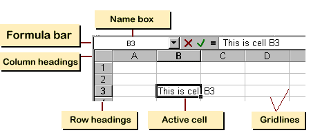
Parts of a worksheet
Terms
| Columns |
Named with letters in the following pattern: A, B, C,…Z, AA, AB, AC,…AZ, BA, BB,
BC,…BZ, CA,…IA, IB,…IV, which is the last possible column.
|
|
Rows |
Named with numbers from 1 to 65,536.
|
| headings |
The gray buttons at the top of columns and
at the left end of rows
|
| cell |
The
intersection of a column and a row
|
|
cell reference or
relative reference
|
The usual way we refer to a cell,
using the letter of the cell's column followed by the number of the cell's row, like B3 or AD345.
|
| Name Box |
At the top left above the
sheet. Used to display cell references and to give and display cell names.
|
| Formula bar
|
Shows the contents of a selected cell, whether it
is plain text, numbers, or a calculation formula. Sometimes the whole
bar that contains the Name Box and the formula text box is called the
Formula bar. Sometimes just the formula text box is meant.
|
| formula |
Looks
rather like an algebra equation, like =SUM(A4:D7) or =AVERAGE(C3, F5, H10). Most formulas use cell references to get the values to calculate with.
|
| absolute reference |
When you don't want the cell reference to change as things are moved around, you must use an
absolute reference, by putting a $ in front of both the column letter and the row number, like $B$3 or $AD$345.
|
| active cell |
  Has a dark border around it and
the row and column headers are either raised, like buttons, or are colored,
depending on your version of Excel. Has a dark border around it and
the row and column headers are either raised, like buttons, or are colored,
depending on your version of Excel.
This is the cell that receives your keystrokes and commands. You make a cell the active cell
when you select
it, by clicking it or by moving into it with keys. The TAB or the arrow
keys are handy for moving from cell to cell.
|
| enter data |
Select the cell, type your data, and
press the ENTER key. What you typed is now contained in the
cell.
|
| range |
 A
rectangular set of cells, referred to by using the upper left and lower
right cell references with a colon between them, like A1:B2 for the range
illustrated at the right. The absolute reference for the range would be
$A$1:$B$2. You select a range by dragging, for example from the upper
left cell to the lower right cell. As you drag, the Name Box shows the
number of rows and columns that are selected. Once you quit dragging, the
Name Box displays the upper left cell. A
rectangular set of cells, referred to by using the upper left and lower
right cell references with a colon between them, like A1:B2 for the range
illustrated at the right. The absolute reference for the range would be
$A$1:$B$2. You select a range by dragging, for example from the upper
left cell to the lower right cell. As you drag, the Name Box shows the
number of rows and columns that are selected. Once you quit dragging, the
Name Box displays the upper left cell.
|
| gridlines |
The gray lines that form the cells. By default they don't print.
 If
you want to print the gridlines, there is a checkbox in the Page Setup dialog (
| |
). If
you want to print the gridlines, there is a checkbox in the Page Setup dialog (
| |
). |
 Cool feature: If you move the
contents of a cell, any formula that contains a relative
reference to that cell is changed to match the new cell reference. A
very handy feature - most of the time. Cool feature: If you move the
contents of a cell, any formula that contains a relative
reference to that cell is changed to match the new cell reference. A
very handy feature - most of the time.
 Over-writing cell contents: If you select a cell
and start typing, what you type replaces what is already in the
cell! To edit what is already in the cell, double-click the cell.
Then you can use the same editing methods you've used in Word- arrow keys
to move the cursor, BACKSPACE and DELETE keys to remove characters,
etc. This is called "editing in place". You can also select the cell and
then click in the Formula bar and edit there. This is the only way older
spreadsheets will allow you to work with the data. Data was only
displayed in the cell. Typing had to be done in the Formula bar. Awkward! Over-writing cell contents: If you select a cell
and start typing, what you type replaces what is already in the
cell! To edit what is already in the cell, double-click the cell.
Then you can use the same editing methods you've used in Word- arrow keys
to move the cursor, BACKSPACE and DELETE keys to remove characters,
etc. This is called "editing in place". You can also select the cell and
then click in the Formula bar and edit there. This is the only way older
spreadsheets will allow you to work with the data. Data was only
displayed in the cell. Typing had to be done in the Formula bar. Awkward!
 Hidden contents: What happens
when the data in a cell is wider than the cell? The contents of a cell will overlap the cell to the right
if that cell is empty. If
the cell to the right is not empty, what you see in the cell will be
cropped to fit the size of the cell that it is in. None of the
cell data is lost. You just can't see it. Cells A2 and B3 below have text that
overlaps the empty
cells to the right. But A3 shows only what will fit. Compare what you see in
cell A3 to what is in the Formula bar. The Formula bar shows all the text in the selected cell. You will learn what to do about this awkward
situation later. Hidden contents: What happens
when the data in a cell is wider than the cell? The contents of a cell will overlap the cell to the right
if that cell is empty. If
the cell to the right is not empty, what you see in the cell will be
cropped to fit the size of the cell that it is in. None of the
cell data is lost. You just can't see it. Cells A2 and B3 below have text that
overlaps the empty
cells to the right. But A3 shows only what will fit. Compare what you see in
cell A3 to what is in the Formula bar. The Formula bar shows all the text in the selected cell. You will learn what to do about this awkward
situation later.

Triangles in Cell Corners
Microsoft Excel uses small triangles in the corner of a cell to
indicate formula errors, comments, or smart Tag options.
 Error = Green triangle in upper left corner
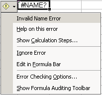 Click
the cell and the Trace Error icon appears. Click the arrow next to the
icon to see a menu of options. Click
the cell and the Trace Error icon appears. Click the arrow next to the
icon to see a menu of options.
 Comment = Red triangle in upper right corner
 Hover
over the cell and the embedded comment appears. Hover
over the cell and the embedded comment appears.
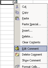 Right
click the cell for a menu that includes choices about the comment. Right
click the cell for a menu that includes choices about the comment.
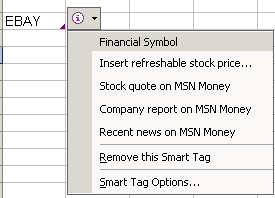  Smart Tag = Purple triangle in lower right
corner
Hover over the cell and the Actions button appears. Click the arrow
to see a menu of Smart Tag options.
|

![]()