
Jan's Working with Numbers
Design: Exercise Excel 5-5
You will use all of the skills and information you have gathered about good spreadsheet design and create your own sheet to show the percentage of total sales in August each ticket type represented.
You have free choice as to the layout and formatting this time! So the results will (should!) vary.
Exercise Excel 5-5: |
Theater Tickets - Subtotals |
| What you will do: | Use the Planning checklist Sort Subtotal Create formulas Create Pie Chart or PivotChart |
Start with: ![]() , ex5-1-theatertickets-Lastname-Firstname.xlsx in folder excel project5 [Created in previous exercise 5-1.]
, ex5-1-theatertickets-Lastname-Firstname.xlsx in folder excel project5 [Created in previous exercise 5-1.]
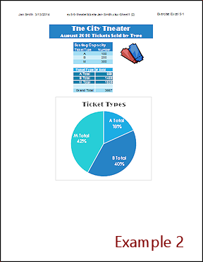
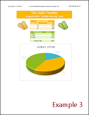
The theater manager wants to know what percentage of
total sales during August each of the ticket types was. In other words, he
wants to be able to fill in the blanks in the following sentence:
Type
_____ tickets were _____% of total sales in August. This compares each
type to the total of actual sales.
You will use the Planning Checklist and construct such a sheet based on ex5-1-theatertickets-Lastname-Firstname.xlsx from your Class disk. You will use Subtotals to calculate how many of each ticket type were sold. You will have to sort first. Then you will create a pie chart to display the results.
-
 Open ex5-1-theatertickets-Lastname-Firstname.xlsx from the excel project5 folder on your Class disk.
 - Save As with the name ex5-5-percentages-Lastname-Firstname.xlsx in the excel project5 folder of your Class disk.
- Planning 1 Goals- In a Comment in cell A1, state the
goals for the sheet.
- Planning 2 Input/Output- In the Comment in cell A1, identify
the output wanted and the input and formulas required.
- Planning 3 Layout- Make changes to the layout and formatting
so it will be easy to read and so that the percentages that the manager wants
to see are especially obvious. Remove from the final version of the sheet the parts of the
original that are not used, such as the play names and dates. Change the
subtitle.
Hints:
1) From the second of the three tables you only need the data in the columns Ticket Type and # Sold.2) The original sheet created subtotals for each play. Remove those totals and the grand total and use Excel's Subtotals feature to create subtotals for each type of ticket. Remember to Sort first. Show only the type totals.
4) Create the a pie chart of the percentages on the same sheet.
- Planning 4 Test- Test your calculations by making a copy to Sheet3 and change the numbers on that
sheet - easy numbers, realistic numbers, and special numbers.
- Planning 5 Documentation - Document your design
choices using comments in appropriate cells. Have all the comments print at
the end.
- Prepare to print: Create a header with your name and the date on the Left, the filename and sheet name in the Center, and Exercise Excel
5-5 on the Right. Spell Check. Print Preview. (All
comments should print at the end.)
- Save.
[ex5-5-percentages-Lastname-Firstname.xlsx]
-
 Print the sheet.
Your print-out should show the table of values and the pie chart on one page and the comments on a second page. [Results will vary, of course.]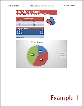
|
|
| © 1997-2017 Jan Smith All Rights Reserved |
Site Map What's New |
Privacy Policy Terms of Service Copyright Acknowledgements |
~~ 1 Cor. 10:31 ...whatever you do, do it all for the glory of God. ~~
Last updated: March 22, 2017
This exercise uses the document from Exercise 5-1. Save the changed document to your Class disk in the excel project5 folder. This keeps the original files intact in case you need to start over.