Jan's Working with Numbers
Design: Logical Tests: Conditional Format
A special use of a hidden IF function is to create formatting that depends on certain conditions - conditional formatting. Combining different values and different formats based on a logical comparison can make your sheet super cool! And informative!
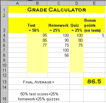
For example, in the Grades Calculator, when the Final Average is under 70, you could change the formatting of the Final Average. You could have different formatting if the grade dropped below 60, a failing grade.
![]() Click on the illustration to see conditional formatting in action. An IF function
adds appropriate text and
conditional formatting changes the look of the Final Average cell. These combine to point out dangerously low grades.
Click on the illustration to see conditional formatting in action. An IF function
adds appropriate text and
conditional formatting changes the look of the Final Average cell. These combine to point out dangerously low grades.
IF function and conditional formatting
point out low grades
Visualize Data with Conditional Formatting
Excel's Conditional Formatting button makes it easy to format a cell based on the value in that cell. You can use the menu choices or write your own rule. When you want to change a cell depending on the value of a different cell (not comparing the cell to that other cell), you must write your own rule.
There are also several schemes for adding visual indicators to your data - a bar, a color, or an icon. These schemes are all based on the value in the cell and compare it to other values in the range.
You must tell Excel to which cells you want to apply the conditional formatting rule.
|
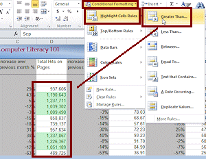
Highlight Cell Rules The illustration shows the effect of a rule for highlighting
values larger than one million. |
  |
|
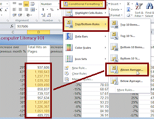
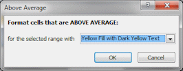
Top/Bottom Rules The illustration shows the effect of a rule that highlights cells whose values are above the average of the column. |
  |
|
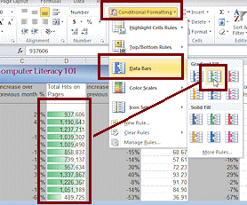
Data Bars In the illustration, the longest bar is for 1,337,867. The shortest bar is for 489,725 which covers about 37% of the cell width because the cell's value is about 37% of the largest value. |
 |
|
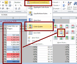
Color Scales The illustrations shows the scheme Red - White - Blue. The
largest value is red; the smallest value is blue. Values halfway
between are white. Other values are shades that are between the
fixed colors. |
 |
|
Icon Sets The illustration shows a 5-icon set, with an up green arrow for the largest value, a down red arrow for the smallest value, and an angled yellow arrow for three stages in between. Other icon sets may have more or fewer stages. |
|
|
Custom Rule If you pick the colors and fonts from the Theme, then they will change when you change the theme. The pre-designed formats do not change when you switch themes. |
 |
| |
Step-by-Step: Conditional Formatting |
|
| What you will learn: | to create conditional formatting to create conditional formatting by formula to test conditional formatting to change the theme to see how it affects conditional formatting to use the sheet to find cells that have conditional formatting |
Start with: ![]() trips35-Lastname-Firstname.xlsx(saved in previous lesson)
trips35-Lastname-Firstname.xlsx(saved in previous lesson)
Format Cells: Conditional Formatting
You will use conditional formatting to give the TotalPoints and Bonus cells different formatting when there is a bonus, and leave the formatting you already applied when there is no bonus due.
-
 Open trips35-Lastname-Firstname.xlsx and select the Bonus sheet, if necessary.
-
 Save as trips36-Lastname-Firstname.xlsx in the excel project5 folder of your Class
disk.
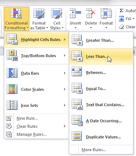
 - Select cell TotalPoints (D11) and from the Home ribbon tab, click the button Conditional Formatting
A drop list of pre-designed rules appears. - Hover over Highlight Cells Rules to expand the choices.
- Click on Less Than...
The Less Than dialog appears with the current value of D11 filled in.
-
 Set
Condition: Set the value to 50 and leave the formatting at the default, Light Red Fill with Dark Red Text.
 - Click OK again to close the dialog.
When this condition is not met, you will see the original formatting. -
 Save.
Save.
[trips36-Lastname-Firstname.xlsx] - Test your new rule by changing the Tahiti trips tickets to 0 and press ENTER.
The total number of points changes to 47 and the cell gets the new conditional formatting. - Undo the value change (but not the conditional formatting).
 Copy
conditional formatting: You can copy conditional
formatting with Format Painter or with Paste Special > Formats, BUT you get
ALL the formatting, not just the conditional formatting rule. Sometimes it's
worth doing even if you have to repair other parts of the formatting.
Conditional Formatting by Formula
What you really need for this sheet is to format the cell Bonus based on the value of a different cell, TotalPoints. That requires creating a formula and doing a custom format.
The new drop list for conditional formatting is cool and useful but it's made it less than obvious how to do a rule like this one!
-
 While
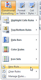
cell G9 Bonus is selected, open the Conditional
Formatting list again and select New Rule...
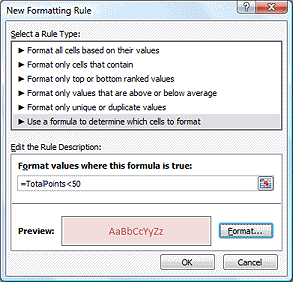
The New Formatting Rule dialog opens.
-
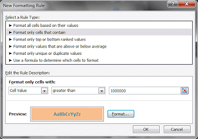
Click on the type Use a formula to determine which cells to format.
-
In the text box at the bottom, type =TotalPoints<50
This is the formula. Looks odd, doesn't it!
You must start with = and then you can write a condition that uses values from other cells.
-
Click on the Format button.
The Format Cells dialog appears. -
On the Font tab, change the Color to the darkest version of Accent 2, which is either a red or an orange, depending on your version of Office.
-
On the Fill tab, change the Color to the lightest version of Accent 2.
These colors are not exactly like the ones in the pre-designed formatting you used for the Bonus cell. They are the closest choices that use Theme colors.
-
 Save.
Save.
[trips36-Lastname-Firstname.xlsx]
Test New Conditional Formatting
-
 Test
< 50: Change some of the trip numbers to change the TotalPoints to
less than 50.
 Test
= 50: Use numbers that will give exactly 50 points.
Does the formatting change as planned in both cases? (This is super cool!)
 Test
> 50: Put in numbers that make TotalPoints greater than 50
- Undo your changes.
Change Theme
It's a good idea to see what effect changing the document theme will have on your carefully selected conditional formatting. The formatting you applied to the Bonus cell will change since you use Theme colors. But the formatting for the TotalPoints cell was from the pre-designed choices. What will happen to it? Let's go look!
- If necessary, open the Clipboard pane again at the left of the window.
This will move the table over so that the themes gallery does not completely cover it.
- On the Page Layout tab, open the Themes gallery and hover over various themes.
Look at what happens to TotalPoints and Bonus as Live Preview shows the effects of different themes. - Change the values for trips to
make TotalPoints less than 50.
-
Repeat the Live Preview of different themes.
What happens to TotalPoints and Bonus? They do not change in the same way. The font changes for both but the TotalPoints cell does not change its font color or background color when you change the theme. All of that changes in the Bonus cell.You could have created a custom format for TotalPoints for the Less Than dialog instead of accepting Light Red Fill on Dark Red Text. In the drop list for that dialog, Custom Format opens the Format Cells dialog.
- Undo your changes of the values.
Use the Bonus Calculator
-
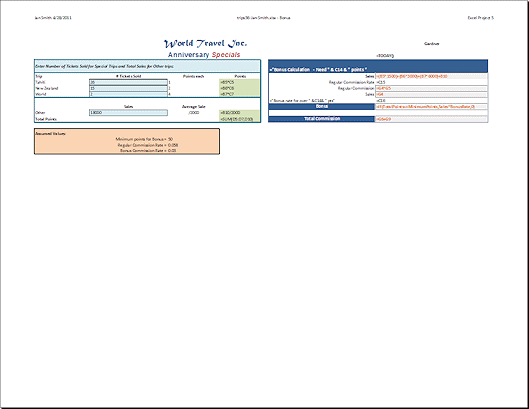 Header: There should already be a header to the Bonus sheet - your name and the date in
the left section, the file name - sheet name in the second section,
Excel Project 5 in the right section.
 - Gardner: With Gardner's data back in place, show the formulas. (CTRL +
` or on the Formulas tab, Show Formulas button.) Widen column
G as needed to show complete formulas.
 Print the sheet on one page in Landscape orientation. Do not print the comments.
After printing, hide the formulas and resize column G to its original width, 77 pixels.
-
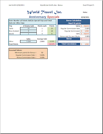 Heinz: Change the name in cell G1 to Heinz.
Fill in the trip numbers for Heinz.
(Use the values on the sheet Specials like you did for Gardner to figure out what he sold.)Heinz does not qualify for the bonus.
 Print page 1 in Portrait orientation, without formulas.
Do not print the comments. -
 Save.
Save.
[trips36-Lastname-Firstname.xlsx]
Find Cells with Conditional Formatting
How can you tell later which cells have conditional formatting? Many cells might have your conditional formatting applied, but not show any format changes because the conditions are not met at this time.
There is a way to highlight these cells, but it will take a few clicks.
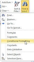
![]() Experiment: Find ALL cells with conditional formatting
Experiment: Find ALL cells with conditional formatting
- Select any cell on the sheet.
- On the Home ribbon tab, at the far right, click the button Find & Select.
A menu appears.Click on Conditional Formatting.
All cells with conditional formatting are highlighted. They may be hard to spot.
Remember that the selected cell has the selection border but not the highlight.
The highlighting changes the colors, but is it enough that you notice the difference? Look for highlighted column and row headers.
- Use the Find & Select menu to find all of the cells with formulas (which include the concatenation formulas), all of the cells with comments, all of the cells with data validation, all of the cells with constants. How easy is it to see which cells are selected? Remember to look at the row and columns headings!
![]() Experiment: Find cells with the SAME conditional formatting
Experiment: Find cells with the SAME conditional formatting
Select a cell with the formatting you want to match.
- On the Home ribbon tab, at the far right, click the button Find & Select.
A menu appears.- Select Go To Special...
The Go To Special dialog appears.- Click on the radio button for Conditional formatting AND the radio button for Same under Data Validation.
- Click on OK.
You cannot try this one unless you add a conditional format to several cells. So far the sheet has two different conditional formats.
Close trips36.xls when you are done.
