Jan's Working with Numbers
Design: Logical Tests: Using IF
The IF function is a real help when you would like to have your sheet behave in different ways depending on the values involved.
For example, in the Grades Calculator below, when the Final Average is under 70, the worksheet shows something special to warn of a low grade. It shows something different if the grade is below 60, a failing grade.
![]() Click on the illustration. An IF function adds some text to cell E14 based on
the value of the Final Average.
Click on the illustration. An IF function adds some text to cell E14 based on
the value of the Final Average.
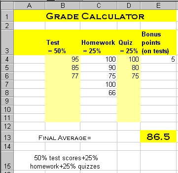
IF function adds text
Formula with the function IF
The IF function produces one of two possible values, based on whether a comparison statement is TRUE or FALSE. A value can be a number, text within double quotes, a cell reference, or a formula.
Syntax of an IF function:
=IF(logical comparison, value if TRUE, value if FALSE)
More than 2 values: You can nest up to 64 IF statements to handle more than two values. For example, you can show three different results by using an IF statement as the "value if False" part.
=IF(E13>100,"Extraordinary",IF(E13=100,"Perfect","Your Average"))
The statement above shows 3 different results, depending on whether E13 is greater than 100 ("Extraordinary"), equal to 100 ("Perfect"), or less than 100 ("Your Average").
| |
Step-by-Step: Using the IF function |
|
| What you will learn: | to write an IF function to name cells to use the Function Arguments dialog to use cell names in a function |
Start with: ![]() trips34-Lastname-Firstname.xlsx (saved in previous lesson)
trips34-Lastname-Firstname.xlsx (saved in previous lesson)
A bonus is not awarded to a travel agent unless the Total Points is 50 or larger. The Bonus Calculation table should not even calculate the bonus if Total Points is less than 50. You can use an IF function to handle this situation.
Formula: IF
What you want to see: If the travel agent earned enough points (50 or more), show the bonus amount. If not, show zero.
- Open trips34-Lastname-Firstname.xlsx and select the Bonus sheet, if necessary.
- Select cell G9, which calculates the Bonus amount, =G4*G8.
-
In the Formula bar write =IF(D11>=C14,G4*G8,0)
 Be careful. Punctuation is critical in a formula! Parentheses enclose the three arguments for the IF
function. The language Excel thinks you are using makes a difference. In English the parts are
separated by commas. In Spanish, for example, semicolons separate the
parts.
What it means:
If Total Points (in D11) is equal to or larger than the minimum number of points needed for a bonus (in C14), the cell will calculate the bonus (multiplying the Bonus Rate in G4 by Sales in G8). If Total Points is not large enough for a bonus, the cell value is zero.In Accounting format you will actually see $ - instead of 0 .
-
 Save as trips35-Lastname-Firstname.xlsx in the excel project5 folder of your Class
disk.
 - Test the formula by changing numbers for the trips to reduce the Total Points below 50.
- Test values that give exactly 50 points also.
- Undo your changes but not the formula change.
Cell or Range Names
The formula in cell G9 would make more sense with words. Who can remember which cell references are which? You will name the cells used in the formula and rewrite the formula to use the names. You can use these names in calculations throughout the workbook.
About Names:
- Names created by typing in the Name Box must be unique to the workbook, not just the worksheet.
- The Name dialog allows duplicate names on different sheets. You must be very careful about how you handle this to avoid errors!!
- Names cannot contain spaces. Allowed characters are letters, numbers, underscore, backslash, and period.
- A name must start with a letter, an underscore,
or back slash character and can have up to 255 characters. (Why
would you use so many??)
In particular, this means you cannot start a name with a number, no matter how logical that might be! - You cannot use a cell reference as a name or the characters C, c, R, or r. Those refer to columns and rows.
- Upper case and lower case characters are the
same. BONUS, bonus, Bonus, and BoNuS are all the same to Excel.
 Be careful to type in the Name Box to name a cell or range and not in the
Formula bar or in the cell itself.
- Select cell D11.
- Click in the Name Box, type TotalPoints ,
and press ENTER to name the cell.
(Remember: you cannot use a space in a cell or range name.)

- Select cell C14 and name it MinimumPoints.
- Select cell C15 and name it CommissionRate.
- Select cell C16 and name it BonusRate .
- Select cell G4 and name it Sales .
- Select cell G9, name it Bonus .
- Check your typing by clicking in each named cell and
looking at what shows in the Name Box.
-
 Save.
Save.
[trips35-Lastname-Firstname.xlsx]
Advantage of using Cell Names:
- The formula actually explains itself if you choose the names wisely.
Disadvantages of using Cell Names:
- You do not see the cell reference that matches the cell name.
- You must spell the name correctly.
![]() Match
labels and cell names: Label each named cell and use the same words as the cell's name in the Name Box. For example,
instead of Minimum points for bonus in cell B14, you could use Minimum Points, which is
nearly the same as the name for cell C14 MinimumPoints. It can help you
later when you've forgotten exactly what you did.
Match
labels and cell names: Label each named cell and use the same words as the cell's name in the Name Box. For example,
instead of Minimum points for bonus in cell B14, you could use Minimum Points, which is
nearly the same as the name for cell C14 MinimumPoints. It can help you
later when you've forgotten exactly what you did.
![]() Problem:
You typed the name in the cell instead of the Name Box.
Problem:
You typed the name in the cell instead of the Name Box.
Solution: Immediately click Undo
and try again.
![]() Problem:
You named
the wrong cell or spelled the name incorrectly
Problem:
You named
the wrong cell or spelled the name incorrectly
If you named the wrong cell,
you cannot just name the right cell with that name. The name is already in
use! You cannot delete it from the Name Box list directly. Frustrating!
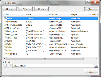
There is a way, however, to correct your mistake - the Name Manager dialog.
 Solution: From the ribbon on the Formulas tab in the Defined Names tab group, click the button Name Manager.
A dialog appears that
lists all the named cells and ranges in the entire workbook, including
print areas and tables. Notice that the references include the sheet name
followed by an exclamation point and the cell references are absolute
references with dollar signs, like =Bonus!$G$9
Just select the name that was
given to the wrong cell and edit the text box at the bottom to change the
cell reference. Or
you can delete the name from the list with the Delete button.
Formula: IF Dialog
Excel knows that some of us are challenged when it comes to proper spelling and punctuation for formulas. There is a dialog method for creating functions that lets you just fill in the blanks. Such a relief!
You will use the dialog to re-write the formula for Bonus to use the new cell names. Formulas make so much more sense with words.
- In the Name Box type Bonus
The cell named Bonus is selected. 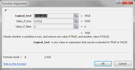 While
the cell Bonus is selected, click on
the
Paste Function button
  .
.
The IF dialog appears, showing the current arguments for the IF statement.
 Problem:
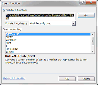
A different dialog opened.
If the cell does not already have a formula in it, a dialog appears that lists all the functions that Excel knows. You can select the function you need from the list.
Solution 1: Cancel the dialog. Click in the correct cell. Click the Insert Function button again.Solution 2: If you clicked the correct cell, you must have lost your formula long the way. Select the IF function from the list.
-
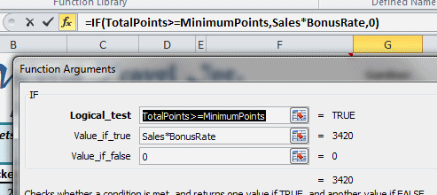 Replace the arguments, using the new cell names:
Logical test: TotalPoints>=MinimumPointsValue if true: Sales*BonusRate
Value if false: 0
Notice that the dialog show you the current value of each of the arguments to the right of the text box for that argument. Make sure these are correct! Of course you must know what those values should be right now. If some of the cells used don't have values yet, you will get errors. It is better to define and name cells before writing formulas that refer to them. If you type a cell or range name incorrectly, you will see an error at the right, like #NAME?
-
Click on OK to apply your changes and close the dialog.
The value of the Bonus cell should not change! Problem:
Cell shows error #NAME?
You have either mistyped the formula or else the name when you named a cell.
Solution: Check your typing in the formula and fix it in the Formula bar. If the formula looks correct, check the names of the cells used in the formula and repair them with the Name Manager on the Formula ribbon tab.
-
 Save.
Save.
[trips35-Lastname-Firstname.xlsx]
Test Formula with Named Cells
Whenever you make a change to a formula, you need to test it all over again.
-
 Test: To
make the total of points less than 50, change C5 to 0 and click the
check mark button on the Formula bar.
The Bonus amount in cell C9 changes to zero. Exactly right! Your formula passed the test!If your formula did not pass the test, repeat the steps in the section above and make corrections.
- Undo your changes to data to get back to Gardner's numbers!
