
Jan's Working with Numbers
Intro: Select & Navigate: Views
There are several different ways of viewing an Excel worksheet. Each helps you work most easily in specific situations. Most are found on the View ribbon tab. (Logical!) In addition, Zoom works in all the views to enlarge or reduce what you see on your screen.
View Choices
All views listed below have buttons on the View tab except Print Preview and Full Screen in Excel 2013 and 2016. There are also buttons at the bottom right of the Status Bar for the three views that are used the most: Normal, Page Layout, and Page Break Preview.
View ribbon tab > Workbook Views tab group
-
 Normal - The default view. Shows gridlines
and headings for columns and rows. Continuous grid.
Normal - The default view. Shows gridlines
and headings for columns and rows. Continuous grid. -
 Page Layout - Lays the Normal view onto sheets of
paper. You can see the page
margins, header, and footer. You can also see parts of the sheet that
won't actually print, if you have set a print area. So this is not
exactly the same as Print Preview. You can edit in this view.
Page Layout - Lays the Normal view onto sheets of
paper. You can see the page
margins, header, and footer. You can also see parts of the sheet that
won't actually print, if you have set a print area. So this is not
exactly the same as Print Preview. You can edit in this view. -
 Page Break Preview - A reduced view of the sheet with blue lines marking what will actually
print and where page breaks occur. You can drag the lines to change
the breaks or to change the print area to keep parts from printing.
Page Break Preview - A reduced view of the sheet with blue lines marking what will actually
print and where page breaks occur. You can drag the lines to change
the breaks or to change the print area to keep parts from printing. -
 Custom Views - A saved combination of column and row sizes, hidden
columns and rows, page breaks, print settings. A custom view is saved with
the sheet. It can only be
applied to the sheet that was active when the view was created.
Custom Views - A saved combination of column and row sizes, hidden
columns and rows, page breaks, print settings. A custom view is saved with
the sheet. It can only be
applied to the sheet that was active when the view was created. - Full Screen -

 Excel 2007, 2010:
Hides the ribbon and Status bar and enlarges the current view to cover the whole screen except for the Windows Taskbar. The ESC key turns off Full Screen view.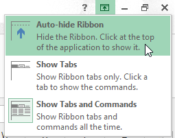

 Excel 2013, 2016:
There is no Full Screen button on the View ribbon tab and ESC does not work to turn off Full Screen view either. So sad.Instead, click the Ribbon Display Options button
 at the top right of the Excel window. Then click on Auto-hide Ribbon. This automatically maximizes the window and hides the Status bar as well as the Title bar and ribbon.
 To turn off this view, you must select the Ribbon Display Options button again and choose one of the other options. These commands do NOT toggle on and off. You must deliberately select the one you want.
View ribbon tab > Window tab group
The choices in the Window tab group are not exactly 'views' but two of them seriously affect how your sheet looks and behaves! We will include Freeze Panes and Split in this list of views.
-
 Freeze Panes -
Fixes part of
the sheet in place while allowing the rest of the sheet to scroll. This lets
you keep the column and row labels in view while moving to areas of the
sheet that are far away.
Freeze Panes -
Fixes part of
the sheet in place while allowing the rest of the sheet to scroll. This lets
you keep the column and row labels in view while moving to areas of the
sheet that are far away. -
 Split -
The button divides the screen into
four panes, so you can view different parts of a large sheet at the same time.
Click the button again to remove the splits. In Excel 2007 and 2010, you can create just two panes by dragging the
Split box on a scrollbar. Excel 2013 and 2016 do not have these split boxes.
Split -
The button divides the screen into
four panes, so you can view different parts of a large sheet at the same time.
Click the button again to remove the splits. In Excel 2007 and 2010, you can create just two panes by dragging the
Split box on a scrollbar. Excel 2013 and 2016 do not have these split boxes.
Print Preview
-
 Print Preview - Shows how sheet will print. This
one is not on the View tab. Excel 2007: Office button menu
Print Preview - Shows how sheet will print. This
one is not on the View tab. Excel 2007: Office button menu  > Print > Print Preview
Excel 2010, 2013, 2016: File tab > PrintUnlike earlier versions, you cannot edit in Print Preview in Excel 2007, 2010, 2013, or 2016.
| |
Step-by-Step: Views |
|
| What you will learn: | to switch to a different view with Status bar buttons to keep part of a sheet from printing with Page Break view to add a header with an automatic date in Page Layout view to toggle Full Screen on and off to split the view into 4 parts to split the view into 2 parts to freeze panes to keep column and row titles in view to open Print Preview |
Start with: ![]() budget-2010-Lastname-Firstname.xlsx from resource
files
budget-2010-Lastname-Firstname.xlsx from resource
files
You will not be saving any changes in this lesson but your instructor may want you to capture some screen shots to prove you did the lesson. Ask.
View: Normal
-
If necessary, select the View tab and click on button Normal
.
Alternate method: Click the Normal view button at the right of the Status Bar.

Normal View displays the document with the grid lines in gray. This is the default view.
In Normal view you may see a dotted line between rows or columns to show where a page break falls. Such a line is hard to see and only shows after you have viewed the document in a way that shows how it fits on paper and then return to Normal view.
View: Page Layout
-
On View tab, click the button Page Layout.
Alternate method: Click the Page Layout view button at the right of the Status Bar.

Page Layout shows how the spreadsheet will fit on paper. It is not a Print Preview because you can add a header or footer. Just click in the header or footer area and type or insert what you want. You can also edit what is in the cells.
 Leave
header/footer to change view. While your cursor is in the
header or footer, you cannot change the view or do anything to the
rest of the worksheet. To get out of the header or footer, just click somewhere in the grid area.
Leave
header/footer to change view. While your cursor is in the
header or footer, you cannot change the view or do anything to the
rest of the worksheet. To get out of the header or footer, just click somewhere in the grid area.
- Scroll the window to see the pages that will
print.
The Status Bar shows that there are 4 pages.
-
 Click at the top of a page, where it says "Click to add header".
The cursor shows up in the center of a text box. The Header & Footer Tools: Design tab appears.
- If necessary, click on the tab Header & Footer Tools: Design
- Type your name and a space.
- Click the button Current Date on the ribbon tab.
You don't see the actual date yet! A code is inserted that will update for the current date.
-
 Click out of the header.
The Header & Footer Tools tab closes and the code changes to show today's date.
-
 Switch back to Normal view.
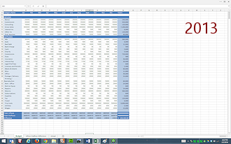
The header you just created does not show in this view. Normal view shows just the sheet data but now has a dashed line to show where the page breaks fall.The illustration shows the worksheet zoomed to show all cells with data.
View: Page Break Preview
-
On the Status bar, click the button Page Break Preview,


 .
.
A message may appear that explains this view.
Alternate Method: On the View ribbon tab, click the button Page Break Preview
.
 Click on OK to close the Welcome dialog, if it appeared.
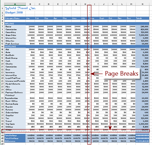
The Page Break Preview uses wide blue lines to show what parts of the worksheet that will print on the same page.
Pages are labeled with large gray numbers (that won't print) in the center of each page area so you can see what order the sections of the worksheet will print. The size of the gray text depends on the the size of the area.
For large sheets with many rows and columns, it can get confusing as to what parts will print on which pages and in what order.
Notice that we don't see the page header in this view.
You can zoom this view, scroll, and even edit.
-
Drag the bottom blue line up underneath Row 42- Wages.
Now the last 3 rows won't print.
The Print Area (the part that will actually print) shows cells with a white background or the background color that you set. Areas that will not print have a dark gray background, even if you set a background color.
While viewing the Page Break Preview, you can edit the cells, move the blue boundaries, and resize columns and rows to make the results clearer. For example, in the current file, you could drag the blue dashed borders and insert new ones to so that the columns for each quarter would print on a separate page.
Do not change the print area any at this time.
-
 Switch back to Normal view.
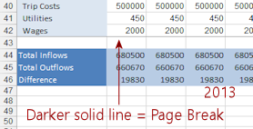
All of the data shows in Normal view but there is a page break line at the bottom of row 42.
Rows 43 - 46 won't print. If they were going to print, you would see a page break line at the bottom edge of row 46.The break line is MUCH harder to see in Excel 2013 and 2016. It is only slightly different from the normal grid lines. Page Break Preview shows the breaks better!
-
 Switch back to Page Layout view.
All of the data shows in this view, too. A dashed line surrounds what will print. Anything outside that will not print!Again, in Excel 2013 and 2016 the line is not dashed and is barely different from the grid lines. VERY hard to notice.
- Switch back to Normal view.
View: Full Screen
For large spreadsheets you may need a larger space to work in. Full Screen View can help with that.
-
Change to Full Screen View:
Excel 2007, 2010: On the View tab click the button Full Screen . Excel 2013, 2016: Click the button Ribbon Display Options
at the top right of the window and then click on Auto-hide Ribbon.
The window automatically is maximized and the ribbon is hidden.
The view expands to take up the whole monitor screen except for the Windows taskbar at the bottom. The ribbon and Status bar for the Excel window go into hiding.
- Return to Normal View:
Excel 2007, 2010: Press the ESC key.
Your screen returns to the previous view.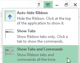 Excel 2013, 2016:Click the button Ribbon Display Options and click on Show Tabs and Commands
Your screen returns to the previous view.
View: Split
Sometime you need to see widely separated areas of a sheet at the same time. You can split the screen into 2 or 4 panes that you can scroll separately.
The Split button on the View tab automatically divides the CURRENT window into 4 equal panes. In Excel 2007 and 2010 there are also horizontal and vertical split bars which create just 2 panes. If you resize the window, the 4 panes do not resize.
-
On the View tab click the button Split.
A Split View with four panes is created.
-
 Experiment: Custom Splits Excel 2007, 2010:

 Drag the Split boxes on the vertical and horizontal scroll
bars to create other split views.
Drag the Split boxes on the vertical and horizontal scroll
bars to create other split views.
(Watch out! There is similar box at the end of the sheet tabs which resizes the space for tabs.)New scrollbars appear. You now have 2 vertical scrollbars and 2 horizontal scrollbars.
- Scroll using each of the scrollbars. What stays in place? What moves.
- Select a range and scroll some more to see
which panes your selection shows up in.
A selected cell or range will show as selected in any pane in which it is visible.
Excel 2013, 2016:
-
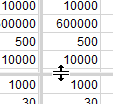
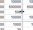 Drag the split bars to resize
the panes.
Drag the split bars to resize
the panes. - Scroll using the scrollbars to see what moves with which scrollbar. If your mouse has a scroll wheel, you can only scroll vertically with it. For a horizontal scroll, you must use the horizontal scrollbar.
- Resize the window larger and smaller.
What happens to the scrollbars?
- Remove the splits by clicking the Split button on the View tab again.
View: Frozen Panes
Frozen panes do not scroll while the rest of the sheet does. This effect is used primarily to hold labels for the rows and/or columns in place while you scroll to the part of the sheet you are interested in. Without the labels it can be hard to tell what you are looking at.
- Scroll the window vertically until row 4 is out of sight.
Is it easy to tell what these columns mean without the labels?
- Scroll the window horizontally until column A is out of sight.
Is it easy to know what these rows mean without the labels? - Select row 5.
-
 On the View tab click the Freeze Panes button.
A menu with three choices appears. The first choice freezes the rows above the selected cell and the columns to the left of the selected cell.
-
Click on the first choice, Freeze Panes.
The rows above your selected row are frozen. Since you selected the whole row, no columns are frozen.
- Scroll up and down.
The top four rows of the sheet stay put!
-
 Unfreeze the pane: Click the Freeze Pane button again and
select Unfreeze Panes.
Unfreeze the pane: Click the Freeze Pane button again and
select Unfreeze Panes.
- Select Column B and then freeze the panes. The
columns to the left of your selected column are frozen.
- Scroll left and right. The first column remains in place.
- Unfreeze the panes.
- Select cell B5 and freeze the panes.
The rows above and the column to the left are frozen.
- Scroll up and down and also left and right. The top and left
of the sheet remain in place so you can see the labels. Very useful on large
sheets.
- Unfreeze the panes.
View: Print Preview
There is no button for Print Preview on the View tab. Unexpected!
Excel 2007 and Excel 2010, 2013, 2016 handle Print Preview differently. All of these versions can have a Print Preview button on the Quick Access Toolbar. (Recommended!)
![]() Remember the No-Print Area: The
bottom rows of the Budget sheet will not show in Print Preview. In Page
Break Preview, we changed the print area to leave them out. If those
rows are included, the print-out takes 4 sheets of paper.
Remember the No-Print Area: The
bottom rows of the Budget sheet will not show in Print Preview. In Page
Break Preview, we changed the print area to leave them out. If those
rows are included, the print-out takes 4 sheets of paper.
- Open Print Preview:
Excel 2007: Clickon
the Office button
 ,
hover over Print to expand its menu, and then click on Print Preview.
,
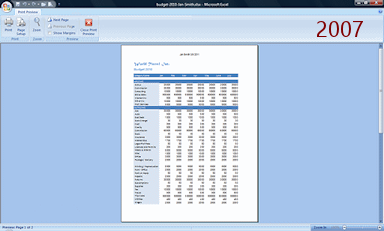
hover over Print to expand its menu, and then click on Print Preview.A print preview window opens, similar to earlier versions of Excel. The Status bar shows that there are 2 pages. You can use the Next Page and Previous Page buttons in the ribbon to see other pages or scroll with the vertical scroll bar. There is a Zoom button at the bottom right if you need to change the size to see better. The header you created earlier shows here on all pages. The cells that you excluded in Page Break Preview are not here.
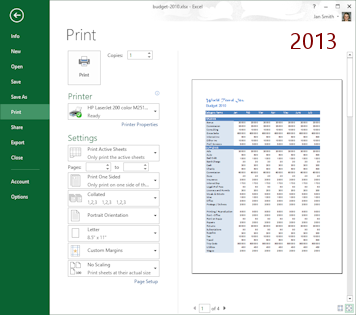
 Excel 2010, 2013, 2016: Click the File tab and then on Print.
 The print preview appears at the right of the Print pane in the Backstage view. The Status bar below the preview shows that there are 2 pages. You can use the arrows at the bottom or the vertical scrollbar to see other pages. The header you created earlier shows here on all pages. The cells that you excluded in Page Break Preview are not here. At the bottom right is the Zoom to Page button
 .
Clicking this button toggles between showing the whole page at once and
showing 100% zoom. You cannot adjust the zoom otherwise. Also at the
bottom right is the button to show/hide margins
.
Clicking this button toggles between showing the whole page at once and
showing 100% zoom. You cannot adjust the zoom otherwise. Also at the
bottom right is the button to show/hide margins  .
Dotted lines shows where the page margins are. You can drag them to new
locations and the document will re-wrap.
.
Dotted lines shows where the page margins are. You can drag them to new
locations and the document will re-wrap.
- Experiment: Print Preview
Try out the choices in the ribbon or pane. What can you change from here? Excel 2007 and Excel 2010, 2013, 2016 are quite different here.
Change the page orientation to Landscape. (In Excel 2007 open Page Setup to do this.)
How many pages will print now? No editing allowed in Print Preview.  Save to your Class disk in the folder excel
project1 with the name
Save to your Class disk in the folder excel
project1 with the name
budget-2010-views-Lastname-Firstname.xlsx
 Print the whole worksheet in Portrait orientation.
[Check with your instructor before printing. There may be special instructions for using your classroom computer or perhaps you need to submit your document electronically.]
|
|
| © 1997-2017 Jan Smith All Rights Reserved |
Site Map What's New |
Privacy Policy Terms of Service Copyright Acknowledgements |
~~ 1 Cor. 10:31 ...whatever you do, do it all for the glory of God. ~~
Last updated: March 27, 2017