
|
Step-by-Step: Conditional Formatting
|
 |
|
What you will learn:
|
to create conditional formatting
to find cells that have conditional formatting |
Start with:
 trips36.xls (saved in
previous lesson)
Format Cells: Conditional
Formatting
With conditional formatting you can have different formatting
for the TotalPoints cell when its value is large enough to qualify for a bonus.
You can change the formatting for the Bonus cell, too. You will make the
TotalPoints
and Bonus cells Green with White text when there is a bonus, and leave the formatting
you already applied when there is no bonus due.
- Select cell D11 and
from the menu select | The dialog opens with the
Condition 1 form ready for you to fill in.
- Set Condition: Fill in the text boxes by choosing: Cell Value Is
and greater than or equal to from the drop lists. Click in the third text
box and type in =$C$14 or just click on cell C14.

 If you do not type the =
yourself, Excel will think you are typing text and will "correct" your entry
to read ="$C$14" , putting quotes around your typing.
This is not what you want!
-
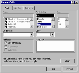 Set
Formatting: Click on the Format… button in the
dialog and choose Pattern | Cell Shading
= Green and Font | Color
= White and Font style = Bold. You do not get quite all of
the Font choices that you are used to seeing in a Font dialog.
-
Click OK to close the Format Cells dialog. The Conditional Formatting
dialog shows a sample using your choices. You can add up to two more sets of
conditions - each with different formatting. This time you only need the one
Condition.

- Click OK again to close the dialog. When this condition is not met,
you will see the original formatting.
- While cell D11 TotalPoints is selected, click the Format Painter
button. Then click on cell G9 Bonus to copy the same formatting to it.
The Conditional Formatting is applied also!
Unfortunately, teal border was also applied to the bottom and right of the
cell and the font size was reduced and you lost the currency formatting. <sigh>
Still, it is often easier to copy a conditional format this way and just fix
any problems that it creates.
-
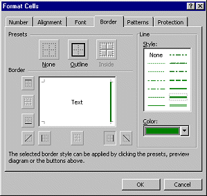 Repair
formatting: With G9 selected, open
| | and change the border to
just a heavy green border on the right and no border on the bottom.
Use the Formatting bar to change the Font Size to 12 and
apply Currency format.
 Save
as trips37.xls
-
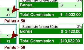 Test: Change some of the trip numbers to change
the TotalPoints to less than 50. Use numbers that will give exactly 50 points.
Does the formatting change as planned in both cases? (This is super cool!)
-
Undo your changes.
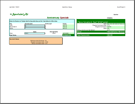
- Gardner:
 With
Gardner's data back in place, show the formulas.
(Tools | Options | View ) Print
the sheet on one page in Landscape orientation. Do not print the
comments. After printing, hide the formulas.
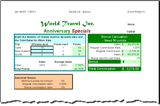
- Heinz:
 Fill
in the trip numbers and name for Heinz and print page 1
in Portrait orientation,
without formulas. Do not print the comments. (Use the
values on the sheet Specials to figure out what he sold.)
Find Cells with Conditional Formatting
How can you tell later which cells have conditional formatting? Many cells
might have your conditional formatting applied, but not show it because
the conditions are not met at this time.
There is a way to highlight these cells, but it will take a few clicks.
To find ALL cells with conditional formatting:
- Select any cell on the sheet.
- From the menu select | | | and
then select Conditional Formatting.
- Click on OK. Cells with conditional formatting will be
highlighted.
To find cells with the SAME conditional formatting:
- Select a cell with the formatting you want to match.
- From the menu select | | | and
then select Conditional Formatting and select Data Validations
- Same.
- Click on OK. Cells with matching conditional formatting will be
highlighted.
Try this with your Bonus sheet. Remember that the selected cell has the
selection border but not the highlight.
Close trips37.xls when you are done.

![]()