|
Facts you need to know:
Tahiti trip = 1 point
New Zealand trip = 2 points
World trip = 4 points
Other trips = points are awarded by dividing
the sales for Other trips by $2000, which is the estimated average
cost of such trips.
Regular commission = 5.8% of sales.
Bonus = an additional 3% of sales, but only if the
agent earns at least 50 points.
You must calculate an agent's number of points earned, the regular commission, the bonus commission, and the total commission.
Design Layout considerations: This
sheet will mostly be used on the screen. So everything an agent needs to see
should fit on one screen at 640 x 480 resolution. (World Travel Inc. uses small
monitors.) The places to enter the number
of trips and sales amounts for Other trips should be obvious. The calculated
values (number of points and commissions) should be easy to tell from the data
entered and the fixed values. The results (Total Points, Bonus, and Total Commission)
should stand out from the other areas.
Printing considerations: The sheet should print on one page in portrait orientation. It should have a place for the agent's name and for the date.
To help keep things organized, you are going to create three tables on the sheet-
-
assumed values table holds the fixed numbers used in the formulas
-
entry table calculates the points
based on the trip info that you enter
-
results table calculates the bonus and total commission

|
Step-by-Step: Create a What If Sheet
|
 |
|
What you will learn:
|
to plan a What-If sheet
to create a table of assumed values
to create an entry table
to create a results table
to use a function to insert today's date
to create a concatenated label |
Start with:
 trips33.xls (saved in
previous lesson)
Remember: To enter a value or a formula you must either press ENTER or click the
 green check mark button after you've finished creating the contents. green check mark button after you've finished creating the contents.
Set Goals; Identify Inputs and Outputs
-
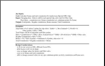 From the facts stated above, on a separate sheet of paper
complete the first two steps of the Planning Checklist for Spreadsheets. From the facts stated above, on a separate sheet of paper
complete the first two steps of the Planning Checklist for Spreadsheets.
[1. Set goals, 2. Identify Inputs and Outputs]
Correct your work later if you find that you left something out. You will use this information to document the sheet in a Comment later.
Design Layout
-
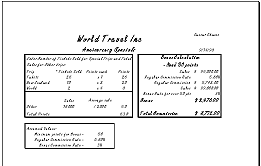 Draw a sketch of a possible layout design for your sheet. It
might be better than what you will be directed to do, which is shown at the
right. When you turn in your work to your teacher, attach the sketch of your
layout. Draw a sketch of a possible layout design for your sheet. It
might be better than what you will be directed to do, which is shown at the
right. When you turn in your work to your teacher, attach the sketch of your
layout.
The parts must be close together to meet the requirement that all fits on one screen at 640 x 480 resolution.
Sheet & Titles
You will create a new sheet for the Bonus Calculator. Remember that you
have to copy the title cells to keep the formatting.
- Open trips33.xls , if
necessary.
- Right click on the sheet tabs and select Insert… and from the dialog select
Worksheet.
- Rename the sheet Bonus.
- Switch to the sheet Tahiti; select cells A1 and A2.
Copy them.
- Switch to sheet Bonus, select cell A1, and Paste.
Customize
- In cell G1 type [Name] . The agent will replace this with his own name.
- In G2 type =TODAY() After the word
TODAY
there is an opening and a closing parenthesis. Each time the sheet is opened, this function will display the
system date, which is the date that the computer thinks it is.
- Format by making both G1 and G2 bold and centered.

Table: Assumed Values
Using a table to hold the constant values used in your formulas makes it easy to change them later if the rules for the bonus change, perhaps for a different set of special offers. Once you have finished this sheet, you
would be able to change the minimum number of points, for example, by changing the value in one place - this table.
-
 Enter Labels & Values: Starting with cell A13, enter the values as in the table to the right. Enter Labels & Values: Starting with cell A13, enter the values as in the table to the right. The text lines below Assumed Values are in column B. They won't look like the illustration just yet.
-
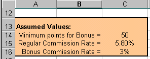 Format: For the table title (cell A13), make
bold. Center the values in cells C14, C15, and C16. Format: For the table title (cell A13), make
bold. Center the values in cells C14, C15, and C16.
Resize the title height by changing Row 13 to a height of 19.50.
For the labels in column B (cells B14, B15, and B16), align right and widen column
B to 14.86, which is just enough to show the entire label and be indented a bit under the title in A13.
Select the whole table (range A13: C16) and fill with Tan background color and
border the whole table with a thick black line.
 Save as trips34.xls . Save as trips34.xls .
Table: Points
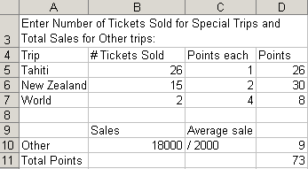
This table is for the data an agent must enter about the number of trips. It
will calculate how many points he has earned. You will fill in the table with
data for Gardner.
-
Enter Labels: Starting with cell
A3 enter the labels as shown in the illustration for the table to
calculate points earned.
For cell C10, you must be in Edit mode or Excel will think this a formula and refuse to let you type the 2000.
-
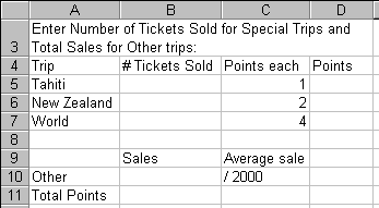 Format: Use to merge across A3 to D3,
wrap the text, left align, and vertical align as Center. Format: Use to merge across A3 to D3,
wrap the text, left align, and vertical align as Center.
Resize Row 3 to show all of the wrapped text. Resize
columns where needed to show the entire label.
Do not AutoFit column B. It would be far too wide because of the labels in
rows 14, 15, & 16.
- Formulas: Values in column D should be calculated by multiplying the value in column B for Tickets Sold by the Points each in column C. So the formula for D5 is =B5*C5 .
Enter this formula and use AutoFill to copy it down to D6 and
D7. All the
formulas result in a zero for now, since there are no values in column B
yet.
The points for Other trips in D10 are calculated by dividing the value in B10 by 2000. Enter the formula for D10 as =B10/2000 . The points will be rounded automatically in General
number format.
The formula for Total Points is in cell D11 is the sum of all the points above. Use
AutoSum and modify the formula.
-
 Enter Data: Switch to sheet
Specials. Find the trips that Gardner sold. Add up the number
of tickets Gardner sold for each trip and also Gardner's total sales for the
Other trips. This is the trickiest part of the project. There is no easy way
to link the data since Gardner has trips scattered around the sheet. Enter Data: Switch to sheet
Specials. Find the trips that Gardner sold. Add up the number
of tickets Gardner sold for each trip and also Gardner's total sales for the
Other trips. This is the trickiest part of the project. There is no easy way
to link the data since Gardner has trips scattered around the sheet.
[Hint: Set AutoCalculate on the status bar to SUM. Select only the cells for Gardner in a group
while holding the CTRL key down. The status bar shows the total.]
Enter the values you found on Specials in the table on Bonus.
Change cell G1 to Gardner .
- Format: To make the places for data entry obvious, border those cells with a heavy black line and fill those cells with
Light Turquoise. (Cells B5, B6, B7, B10) Use the same fill color but no border on the directions in cell
A3. It's nice to coordinate your
colors!
Turn off the display of gridlines. [Tools | Options | View] Now the
borders and fill color clearly show where you are to type in data. (Working
without the gridlines is possible with a small table, but it is not a easy as it
sounds. Another experience for you!)
Format the calculated values differently by filling those cells with Light Green. (Cells D5, D6, D7, D10, D11)
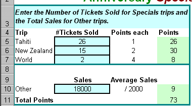 Make the column labels (Cells A4:D4 and B9 and C9) and the row
label Total Points in cell A11 bold. Make the directions in cell
A3 bold and italics. Make the column labels (Cells A4:D4 and B9 and C9) and the row
label Total Points in cell A11 bold. Make the directions in cell
A3 bold and italics.
Center all the columns of data and the calculations (B4:D11).
Select the whole table,
including the directions. Use the Format Cells… | Border dialog to put
a heavy Teal border around it. Then select the directions and
special trips part (A7:D7) and add a heavy Teal border on the
bottom. (You can only get black borders with the button.)
-
Resize Row 3 to a height of 33.75 and Column E to a width of
1.00.
-
 Save.
[trips34.xls] Save.
[trips34.xls]
Table: Commissions
This table will calculate the agent's regular commission, his bonus,
and then add them together for the total commission.
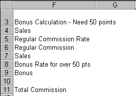
- Enter labels: Starting in cell F3 enter the labels for
the table that will calculate commissions. Widen column F to show the whole
text of cell F8.
Problem - If you change the minimum number of points needed to get the bonus, your
labels will not be updated.
You can fix that!
- Labels that will update: You can mix text
and cell references.
Select cell F3 and edit it to read
="Bonus Calculation - Need " & C14 & " points" . The quotes
around the text and spaces that you want to see are important. The ampersand (&) is used to glue together text and the values in cells, called
concatenation. By using this formula, if the number of points changes,
the label changes automatically.
Select cell F8 and edit this label so the number of points will also update automatically - ="Bonus Rate for over " & C14 & " pts"
- Assumed Values: Link the cells for
Regular Commission Rate and Bonus Rate to the Assumed Values table. You can
more easily see where to change these rates in the future if they are in a
separate table.
For the Regular Commission Rate in cell G5 type
= and click cell
C15 in the table of Assumed Values and
press ENTER.
For the Bonus Rate in cell G8, type
= and click cell
C16 in the table of Assumed Values and press
ENTER.
- Formulas: The easy way to enter these formulas is to type the equals sign and the other symbols, but click on the cell to use.
Sales in cell G4 will require a longer formula than the others. Sales is the sum of the sales for Tahiti, New Zealand, World, and Others. You already have the sales for Others in cell B10, but for the other trips you must multiply the number of tickets by the price per ticket. For example, the Tahiti sales will be the number of tickets times 1500 for each ticket, or =B5*1500.
So your formula for G4 is =B5*1500+B6*3000+B7*6000+B10 . Remember that all multiplications are done before the additions.
If you like, you can add parentheses to make it clearer:
=(B5*1500+(B6*3000)+(B7*6000)+B10
You calculate the Regular Commission by multiplying Sales by the Regular Commission Rate. So in cell G6 you need = G4*G5 Sales is repeated in G7 so you can
see that you are going to multiply it by the Bonus Rate to get the Bonus. So for
G7 you just need =G4 .
The Bonus in cell G9 is the Sales times the Bonus Rate, which is =G7*G8 .
The Total Commission is the sum of the Bonus and the Regular Commission, =G6+G9.
-
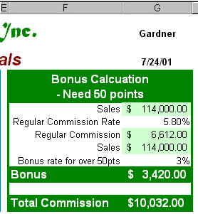 Format: Use the Light Green fill for the calculated values in column G (cells G4, G6, G7,
G9, G11) Format: Use the Light Green fill for the calculated values in column G (cells G4, G6, G7,
G9, G11)Emphasize the title, bonus, and total commission by applying the
cell style Label-white on green to cells F3, G3, F9, G9, and F11, G11.
Use Merge and Center on the title to span F3 and G3. Turn on Text
Wrap in Format | Cells... | Alignment.
To make the title wrap nicely, we need to add a line break in the
concatenated title. We cannot just use the usual key combo. We will have
add to our formula a special code for a line break.
Edit the formula in F3 to include the code for a line break CHAR(10):
="Bonus Calculation "&CHAR(10)&"- Need " & C14 &" points"
(We are getting really technical here! But isn't it cool?!)
  If
the text does not wrap and you see a rectangle after the word Calculation, you
did not turn on text wrapping. If
the text does not wrap and you see a rectangle after the word Calculation, you
did not turn on text wrapping.
Right justify F4: F8. Wide column F if necessary to get all the text
inside the column.
Apply the Currency format to cells G4, G6, G7, G9, and G11.
Select the whole table (F3:G11) and apply a heavy Green border from the Format Cells… dialog.
 Save.
[trips34.xls] Save.
[trips34.xls]
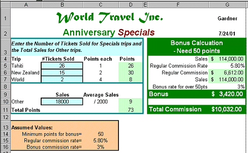
Bonus sheet created
|

![]()