 |
You need to use what you just learned, and maybe learn a little more. Complete all parts of the following exercises. Don't forget to backup your Class disk when you have
completed the exercises or whenever you stop for the day and saved a document
along the way.
|
 |

Where you are:
JegsWorks >
Lessons >
Numbers
Before
you start...
Project 1: Excel Intro
Interface
Select & Navigate
Common
Tasks
Summary
Quiz
Exercises

 Ex. 1: AutoCalculate Ex. 1: AutoCalculate
 Ex. 2: AutoSum, Sort, Format Ex. 2: AutoSum, Sort, Format
 Ex. 3: Chart Ex. 3: Chart
Project 2: Excel Basics
Project 3: Format & Arrange
Project
4: Groups & Formulas
Project 5: Design
Search
Glossary
Appendix
|
|
Exercise Excel 1-2: AutoSum, Sort, & Format
|
What you will do: |
save a copy of a spreadsheet
use AutoSum
sort rows
format numbers
save and print
|
Start with: ,
halfyear.xls from resource files ,
halfyear.xls from resource files
Use the toolbar buttons for AutoSum and sorting to create totals and arrange the rows.
Copy spreadsheet
- From your resource files in the numbers
folder open the file halfyear.xls, or
download the file directly.
 Select from the File menu. In the Save As
dialog, click
 the New Folder button
and create a new folder in the my docs folder: excel
project1. the New Folder button
and create a new folder in the my docs folder: excel
project1.
 Save the workbook as halfyeartotals.xls to the
excel project1 folder.
AutoSum and Sort
- Row Totals: Use AutoSum to create row totals in Column I. After you get two values in Column I, Excel will try to sum the column instead of the row. Change the range when that happens. Remember to press
ENTER to accept the formula.
- Sort: Sort the category rows, Rows 7 - 19, into alphabetical order.
Your formulas refer only to cells in the same row, so you will not mess up
the formulas by sorting. Whew!
- Column Totals: Use AutoSum to create column totals in Row 21. Again Excel will get confused after you have two values in the row. It will try to sum the row instead of the column. Change the range when that happens.
- Grand Total: In cell I22 use AutoSum to create a grand total, but change the range to include all the cells with Light Turquoise background, B7:H20. Type Grand Total = in cell G22.
Format Numbers
- Format currency: Format the new totals in column I and in Row 21 and in cell I22 as Currency.
- Format decimals: There is one value in the table data with a decimal point. Increase the decimals by one for that value.
- Format Painter: Use the Format Painter button to copy the format of cell
E14 to range G22:I22, the grand total and its label. While that range is selected, make the cells bold. Reset I22 to Currency.
- Label sheet: Select cell D1 and type your name and press
ENTER. Select cell E1 and type the date and press ENTER. Select cell D2 and type Exercise Excel
1-2
- Prepare to Print: Switch to
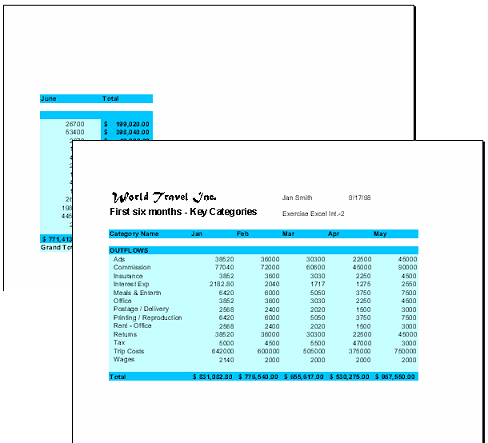
 Print Preview. Check what will print. Make corrections if necessary. This sheet prints on two pages. Print Preview. Check what will print. Make corrections if necessary. This sheet prints on two pages.
 Save.
Save.
 How to handle a full disk How to handle a full disk
 Print. Print.

|

![]()