|
Exercise Excel 4-1:
|
Amazon Pings: Insert and Repair
|
| What you will do: |
Copy and insert data
Print selection
Paste Link
Repair formulas
Copy formatting
Revise chart
Print grouped sheets |
Start with:
 ,
amazon pings3.xls
from Project 3: Ex. 3-3 ,
amazon pings3.xls
from Project 3: Ex. 3-3
Were your formulas in amazon pings3.xls correctly designed to automatically include inserted columns? You will find out now.
-
Open amazon pings3.xls from the
excel project3 folder of your Class
disk.
- Save As with the name amazon pings4.xls
to the folder excel project4.
- Select the sheet Week 2. Note the values in the
Average, Maximum, and Minimum columns and the values in M31:M33, the
cells that are supposed to use all the data cells. You will need these
values later to see if they change.
- Insert Columns: Select on sheet Original Data the data for
the third week (range Q1:W33) and Copy. On sheet Week 2 select cell J1
and Insert | Copied cells. Shift cells to right. This inserts the cells
but they are not linked to the original data, so continue with Paste
Special… | Paste Link. (If you can not paste, the Clipboard lost your
copy. Copy again from Original Data.)
Why this awkward method?
Inserting first creates the columns to Paste Link in. If you try to link
first, you lose the existing columns for Average, Maximum, and Minimum.
- Edit: Change cell G1 and the sheet tab to read Week 2 & 3. Remove the zeros
from the cells that were originally blank. The data cells with zeros
mean that the system was down at those times and no pings were recorded.
Delete those zeros also since they are not real ping times. The Minimum
time can not really be zero!
- Copy table formats: Select column I and Copy. Select columns
J through Q and Paste Special… | Formats.
- Resize: Resize the new columns to 9.57 to match what
AutoFormat did, if necessary.
- Formulas: Are all your formulas including the new cells?
Ranges should go to column Q. Show the formulas. [Hint: Tools | Options]
Revise if necessary.
[If the totals were not updated, then your original
ranges for the formulas did not include the blank column, originally
Column J.]
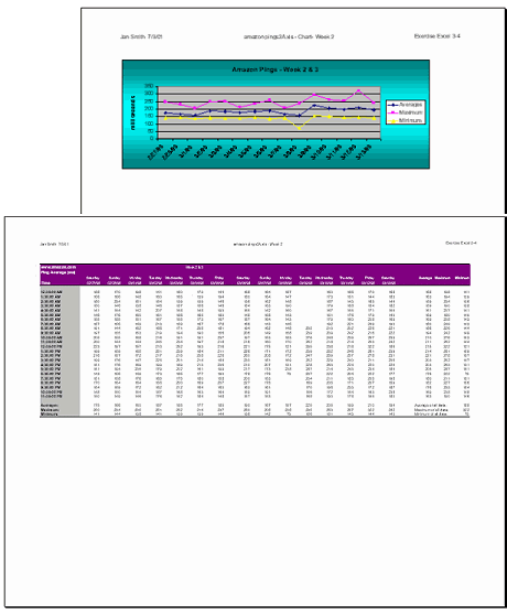
- Chart: Edit the title for the chart to read Week 2 & 3
and the sheet tab to read Chart - Weeks 2 & 3. Drag
the updated chart wide enough to show all the dates along the bottom.
(about as wide as columns A to L)
[If the chart was not updated, then your original ranges for the chart
did not include the blank column, Column J. Select the chart and from
the menu choose Source Data…. | Series. Edit the ranges for Values for
each Series and for Category (X) axis labels to end in column Q instead
of column I.]
- Prepare to print: Edit the headers for the sheets to read
Exercise Excel 4-1. Spell Check. Look at Page Break Preview and Print
Preview. Select sheet Weeks 2 and 3, and under Page Setup | Page, set the
orientation to Landscape and Fit to 1 page wide by 1 page tall. Select
sheet Chart - Weeks 2 and 3, and check under Page Setup | Page that it will print with
Portrait orientation and Fit to 1 page wide by 1 page tall.
-
Save. [amazon
pings4.xls]
- Select the two sheets Week 2 and Chart.
- Print the active sheets. One will be landscape and one
portrait. [If the chart is still selected when you try to print, the chart
will take up a whole page.]
After the printing is
finished, close the workbook.
|