|
Improvements you will make:
- Rework subtitle. A little color will help a lot.
- Remove data in the Trips column since all trips on each sheet are the same.
- Add images to the 4 trip sheets.
Your images will be larger than a single cell.
- Add a title naming the trip covered on each sheet.

|
Step-by-Step: Add Image
|
|
|
What you will learn:
|
that a linked cell can have only 1 format
to insert an image from a file
to move and resize image
to select cells underneath an image |
Start with:
 trips25.xls - sheets for trips
(saved in
previous lesson),
resource files
trips25.xls - sheets for trips
(saved in
previous lesson),
resource files
Format linked cells
Recall that the title cells for all the other sheets
are linked to the title cells on Specials. At one point in you
experimenting the subtitle Anniversary Specials was formatted as
 . That red Specials would look good, but there is a problem because of the
linking. . That red Specials would look good, but there is a problem because of the
linking.
-
Open the sheet Tahiti and select cell
A2, the subtitle Anniversary Specials. The Formula bar shows that
this cell is linked: =Specials!A2 .
-
Switch to Specials and select A2.
-
Format the word Specials as Dark Red and
italic.
-
Switch back to Tahiti. Whoops. The subtitle did not
update to show the new formatting!
Linked cells do not carry formatting with them.
Earlier you applied formatting
with Paste Special. But Paste Special and Format Painter only see
the first formatting in the cell. The red and italics is ignored. <sigh!>
Another approach is needed.
-
Copy cell Specials!A2.
-
Group sheets Agent Totals, Tahiti, New Zealand, World, Other,
and Formatted Groups.
-
Select the sheet Tahiti and paste to A2.
Now all the A2 cells in all the grouped sheets are the same as Specials!A2,
but they are not linked to Specials!A2.
-
Ungroup the sheets.
-
Save
as trips26.xls .
 How to handle a full disk
Remove Trip column data
You are going to remove the data in the Trip column since it is not
needed on the trips sheets. Each sheet is about only 1 trip. You will leave the cells blank instead of
deleting them so there will be some room for an image.
- Group the sheets Tahiti, New Zealand, World, and Other.
- Select cells A4:A11 (this includes all the cells in
column A with data on all 4 sheets). Press DELETE. The Trip
column is now blank. The formatting is still there. Check each sheet in
the group.
- Ungroup the sheets.
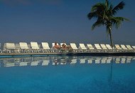
Insert Image: Palm
Now you have some space for an image.
- Select sheet Tahiti.
- From the menu select |
| .
- In the Picture dialog, type the path to the resource files image -
c:\My Documents\complit101\numbers\palmtree.wmf
. The palm tree image is placed on the sheet at its original size,
which is much larger than you need.
Resize & Position Image
- Reduce the size of the image by dragging a corner handle
of the image until it is about 6 rows tall.
- Drag the image to rows 5 - 10 in column A.
- Widen column A to hold the whole tree.
The gridlines behind
the palm tree show because part of the image is transparent. You can get
rid of them by merging the cells under the image.
The trick is how to get the cells selected while the image is on top
of them. You could move the image while you select, but sometimes it is hard to get
an image back just exactly right.
-
 Select
cell A3. Use the arrow key to move down to cell A4, underneath
the image. Hold the SHIFT key down and use the down arrow to move
to A10. Now the range A5:A10 is selected. Select
cell A3. Use the arrow key to move down to cell A4, underneath
the image. Hold the SHIFT key down and use the down arrow to move
to A10. Now the range A5:A10 is selected.
- Click on
 the Merge and Center button. Gridlines are gone!
Insert Image: New Zealand and World sheets
-
 Repeat the
procedure for the sheet New Zealand Repeat the
procedure for the sheet New Zealand
[Insert image NZflag.wmf
; resize image to about 3 rows tall, and position image in column
A; widen column A, merge cells A5:A9.]
- Repeat the procedure for the sheet World, with one additional step.
[Insert image Globe.wmf; resize image to
about 4 rows high.]
- Before positioning the globe image, resize Rows 5 and
6 to 30.00 high.
The globe would be much too small if you make it fit over two rows at
the default height.
(Hint: select the rows and drag a bottom edge of a row heading. Look at the
popup tip for the size.)
- Select rows 5 and 6 and set | | |
= Center.
- Position the globe image in column A.
- Widen column A and merge cells A5 and A6 to remove the gridline.
Format sheet: Other
- Select sheet Other. You don't have
an image for this one, but you can clean it up a bit.
- Select cells A5:A10 and click
the Merge and Center button. Click on OK on the message about losing cell
contents.
- With the merged cell selected, | | |
= Center.
- On the Font tab, set Arial, Bold, size 12,
Green.
- Type Other .
- AutoFit column A.
-
Save. [trips26.xls]
How to handle a full disk
Add Subtitle: Trip
The images give you a big clue and the sheet title clearly tells you
what each sheet is about. Still, when printed or glanced at quickly, the
sheet needs to say plainly what trip is covered on that sheet.
You will add and format another subtitle.
- Group sheets Tahiti, New Zealand, Worlds, and Other.
- Select cells A3:F3, which are between the subtitle
Anniversary Specials and the column labels.
- Click on
the Center and Merge button.
- Click on cell A2 and then on
 the Format
Painter button to pick up the formatting of
the subtitle. the Format
Painter button to pick up the formatting of
the subtitle.
- Click on cell A3 to apply the formatting to the new
merged cell. There is no text there yet.
- Ungroup the sheets.
- On each of the 4 trip sheets, in cell A3 type the trip for that sheet: Tahiti, New
Zealand, World, or Other.
-
Save. [trips26.xls]
How to handle a full disk
|