Jan's Working with Numbers

Exercise Excel 2-2: Soccer Budget

Start with: a blank worksheet

The City Soccer League has created a budget for their season. You will put their figures on a spreadsheet and create formulas for totals and to show whether the league went over the budget.

1. Open a blank workbook and save as ex2-2-soccerbudget-Lastname-Firstname.xlsx in the excel project2 folder on the Class disk.
   
2. Data Entry: Use the handwritten notes in the illustration to create a spreadsheet. Fill in titles starting with row 1, labels, and data in the same order. Leave a blank row above Expenses, below Insurance, one above Income, and one below Sponsorships.

   

   
   
3. Sort: Sort the Expenses rows in alphabetical order. (Don't just sort the words. Sort rows.)
   
4. Resize columns: Widen Column A enough to show the category names.
   

5. Formula: Create a formula in cell D7 (in the first data row- Balls- in the column Over/Under Budget) to subtract the Actual amount in column C from the Budget amount in column B. If the league spent more than planned, the answer will be a negative number. Copy this formula to the other cells in this column that are on rows with categories or totals. (Hint: Copy down the whole column and then delete unneeded values.)

   If necessary, press the F9 key to make Excel recalculate the values.  

6. AutoSum: Use AutoSum to calculate Totals for Expenses and Income in both the Budget and Actual columns.
   Column D should already have a formula to calculate the Over or Under budget amount.
   
7. Numbers: Format the numbers on the sheet as Accounting using the button for range B7:D14, range B16:D16, range B19:D20, range B22:D22. Decrease Decimals twice. Note that the negative numbers now are in parentheses.
   
8. Edit: To explain the new parentheses for negative values, put parentheses around the word Over in the column label: (Over)/Under. Shorten the text in cell B6 to Budget.
   
9. Header: Create a header with your name and the date on the left, the file name and sheet name in the center and Exercise Excel 2-2 on the right.
   
10. Prepare to Print: Use Page Setup to set the table to print centered horizontally on the page but not vertically. No grid lines or headings. Spell Check. Print Preview.
    
11. Save.  
    [ex2-2-soccerbudget-Lastname-Firstname.xlsx]
    
12. Print
    
13. Select the range A1: D16, which is just the titles and Expenses rows.
    
14. Print just the selection.
    
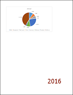
15. Chart: Select ranges A6:A14 and C6:C14 at the same time. Create a pie chart of what was spent. Use the default settings except for Data labels. Change the Data Labels to show Percentage and position Outside End. (Excel 2013, 2016: Create Sheet2) Move the chart to Sheet 2. The chart title should be "Actual". Drag the chart to the upper left of the sheet. Be sure to click off the chart before continuing.
    
16. Chart Header: Create a header for Sheet2 just like in step i. 
17. Prepare to Print Sheet2: Use Print Preview to check the layout and header. If the chart takes up the whole page, it is selected. If the header does not show, then the chart was selected when you created the header. Go back to Normal view and unselect the chart. Create the header again if it did not show.

    If your chart does not show in Print Preview, switch to Page Break Preview and wait for it to show up. Then go back to Print Preview.
    Sometimes Excel takes a while to do some thinking in the background before it can display what you've done.

18. Save.
    [ex2-2-soccerbudget-Lastname-Firstname.xlsx]
    
19. Print. Once the printing is completed correctly, close the workbook.

Excel 2013, 2016: The chart will use different colors and has the legend across the bottom.