
Jan's Working with Numbers
Excel Basics: Getting Started: Sheet
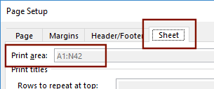
Spreadsheets can be really big. One way to print just exactly the cells that you want is with the Sheet tab in the Page Setup Dialog.
 To print only part of a sheet, you set a Print Area.
Only cells in this Print Area will actually print, no matter what you see on
your screen. The Page Break Preview is better for managing several pages,
but this dialog is good for smaller jobs.
To print only part of a sheet, you set a Print Area.
Only cells in this Print Area will actually print, no matter what you see on
your screen. The Page Break Preview is better for managing several pages,
but this dialog is good for smaller jobs.
The Print Area could be the whole sheet, a range, a single cell, or even several ranges scattered over the sheet. Each separate range would print on a separate page.
If you move the cells in the Print Area, the cell references for Print Area will change to show the new location(s). Handy dandy!
| |
Step-by-Step: Setup Sheet |
|
| What you will learn: | to set the print area using: Page Setup dialog and keyboard Page Setup dialog and mouse Ribbon button and mouse to clear print area to print titles - repeating columns and/or rows to print the spreadsheet |
Start with:![]() ,
, ![]() budget-2010-Lastname-Firstname.xlsx from
previous lesson
budget-2010-Lastname-Firstname.xlsx from
previous lesson
Open Page Setup > Sheet tab
- From your Class disk open your old friend budget-chart-2010-Lastname-Firstname.xlsx.
- If necessary, select the sheet Budget and then open Print Preview.
How many pages will it take to print this sheet?
-
Open the Page Setup dialog from Print Preview.

 Excel 2007: Click on the Page Setup button.


 Excel 2010, 2013, 2016: Click on the Page Setup link to the left of the
preview.
Excel 2010, 2013, 2016: Click on the Page Setup link to the left of the
preview.
-
 Click on the Sheet tab
in the Page Setup dialog.
Click on the Sheet tab
in the Page Setup dialog.
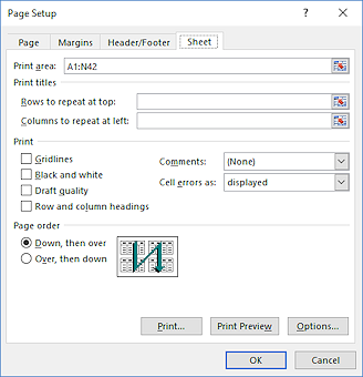
This dialog tab sets options for how the selected sheet will print. Inspect the options on this tab. Not all are available! The Print area
text box is gray. You cannot adjust the print area because you opened the dialog from
Print Preview. How odd!
The Print area
text box is gray. You cannot adjust the print area because you opened the dialog from
Print Preview. How odd! - Close the dialog and go back to the Normal view.
-
 Switch to the Page Layout ribbon tab and then open the Page Setup dialog and click on the Sheet tab.
Now the Print area box is available for changes.
Print area is showing A1:N42 because in a previous lesson while in Page Break Preview you set a print area when you dragged the bottom blue line up to keep the totals rows from printing.
All other check boxes and text boxes should be blank at this time.
Print Area: Dialog with Keyboard
The Print Area is the cells which will be printed. Sounds simple enough. When you know the cell references, it is quick and easy to just type them in.
-
 Type in the Print Area text box the range a1:d4 .
- Click on
 the Print Preview button in the dialog.
Not much will print! Only the cells in the range that you typed, a1:d4, which is just the titles and some labels.
-
 Switch back to Normal view.
Your Print Area is still a1:d4 and has a border around it in Normal view now.
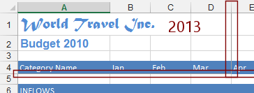 Excel 2013, 2016: The print area is really hard to see. The solid line is only slightly different from the normal grid lines.
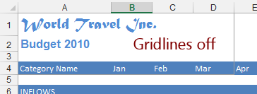
 Tip: On the View ribbon tab, uncheck Gridlines. The right border for the print area is now noticeable but the other edges are still hard to see.
Print Area: Dialog with Mouse
When you don't know the cell references, you can pick out the cells you want to print by clicking or dragging in the sheet itself.
-
Open the Page Setup dialog again to the Sheet tab.
-
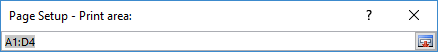 Click on
  the Collapse Dialog button at the right end of the Print Area text box. The dialog collapses to show just the text
box. The button changes to
the Collapse Dialog button at the right end of the Print Area text box. The dialog collapses to show just the text
box. The button changes to  the Restore Dialog button. The collapsed dialog will stay on top while you work in the spreadsheet itself.
If it is still in the way, you can drag it by its Title bar.
the Restore Dialog button. The collapsed dialog will stay on top while you work in the spreadsheet itself.
If it is still in the way, you can drag it by its Title bar.The Collapse Dialog button
appears in all Excel dialog text boxes in which you can enter cell references.
You will use it again!
-
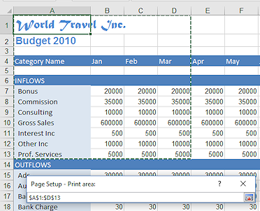 On the sheet Budget, drag from cell A1 to
cell D13.
On the sheet Budget, drag from cell A1 to
cell D13.
This selects the Inflows for the first quarter of the year and the sheet titles.
The absolute references appear in the text box.Notice that the Print Area has a wide line, dashed border. Much easier to see. This depends on cursor being in the Print area text box on the Sheet tab of the dialog.
- Click the Restore Dialog button at the end of the text box to return the collapsed dialog to its original size.
Losing changes: If you close
the dialog with the

 Close button at the top right of its Title bar, all your
changes in that dialog will be lost! You should always restore the dialog first and then click on the OK button to
exit. (Unless, of course, you want to forget all about what you just did!)
Close button at the top right of its Title bar, all your
changes in that dialog will be lost! You should always restore the dialog first and then click on the OK button to
exit. (Unless, of course, you want to forget all about what you just did!)
-
 Click on the Print Preview button.
Only the cells you selected show as printing.Non-adjacent
ranges: You can
select non-adjacent cells and ranges. Their range cell references in the Print area text box
will be separated with a comma, like $E$3:$F$6, $G$15:$I:$89. But each range will
print on a separate page.
The Print Area can also be set by first selecting on the sheet the ranges that you want to print and then choosing File > Print Area > Set Print Area.
- Switch back to Normal view.
Print Area: Ribbon Button
You can also create a print area using a button on the ribbon.
-
 In
Normal view, drag from A1 to G13.
In
Normal view, drag from A1 to G13.
- On the Page Layout tab click the Print Area button to drop its
menu.
- Click on Set Print Area.
-
 Switch to Print Preview.
Now the page shows the Inflows for the first 6 months plus the titles.
- Switch back to Normal view.
Clear Print Area
If you don't want to restrict printing to your Print Area all the time, you need to clear out those cell references. There is an easy way!
-
 Click to deselect the print area you set last.
- On the Page Layout tab click the button Print Area and then Clear Print Area.
You did it! The border lines around the range A1:G13 vanish and Excel recalculates where the page breaks fall to print the whole sheet.
- Switch back to Print Preview one last time to see what will print.
The preview shows all 4 pages, including the Totals rows.
Print Titles: Repeat Rows/Columns
 When your sheet won't fit on just one page, it
is helpful to
have the column and row labels repeat on the following pages. Excel
calls this Print Titles. One of the common
uses for this feature is to include the title of the worksheet on
every page.
When your sheet won't fit on just one page, it
is helpful to
have the column and row labels repeat on the following pages. Excel
calls this Print Titles. One of the common
uses for this feature is to include the title of the worksheet on
every page.
Labels are the text that you typed into cells to explain what the rows and columns are about. If the Print Area won't fit on a single piece of paper, you will have one or more columns of data off on a page by itself. With no labels, this data won't make much sense.
In the Budget sheet, the column labels are in row 4 (months of the year) and the row labels are in column A (category names).
Repeat one column:
- Switch back to Normal view.
- On the Page Layout tab click the button Print Titles
 .
.
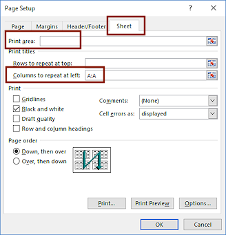
The Page Setup dialog opens directly to the Sheet tab.
The dialog shows the old cell references, A1:N42.
-
If necessary, delete any cell references in the Print Area box.
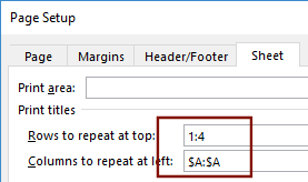
There are two text boxes under Print Title. One for rows and one for columns.
The layout of this Budget sheet has labels for rows in Column A, so that would be a good column to see on every page.
-
Type A in the box Columns to repeat at left and click on OK.
Whoops. A message appears. Excel wants more than just 'A'.
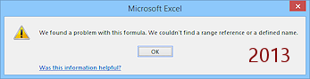
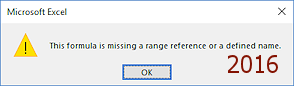
- Click on OK to close the message.
 Replace the A with A:A,
which is the correct cell reference for the whole column.
Replace the A with A:A,
which is the correct cell reference for the whole column.
- Click on OK to close the
Page Setup dialog.
Back in Normal view, nothing has changed. The Sheet tab only affects printing.
-
Switch to Print Preview.
Inspect all pages.The row labels from column A are included on all pages.
Now when you need to look on the print-out at the value for Gross Sales in December (cell M10), you don't have to count down the rows. The row label is right there on the page.
That's better, but pages 2 and 4 don't have column labels across the top. That makes it hard to tell what was being totaled!
Pages 1, 2, 3, 4 with Column A included on each page
Repeat multiple rows:
You can repeat more than just one row or one column. Let's get the column labels and the title and subtitle for the worksheet. We have to use complete rows that are adjacent to each other. You cannot just pick parts of rows or rows scattered around. Think about that when you first plan a worksheet!
-
 Switch back to Normal view and click on Print Titles again.
Did the Print Area show up again?Notice that Excel turned your A:A into $A:$A, absolute references. Apparently that's what Excel has to have to make this work.
- If necessary, delete any cell references in the Print
Area.
- Type 1:4 in the box Rows to repeat at top and click on OK.
Excel turns that into $A$1:$A$2,$4:$4 for you. That's a nice feature!
- Switch to Print Preview yet again.
Pages 1, 2, 3, 4 with Column A and Rows 1 - 4 included on each page
Much more user friendly! -
 Save your file to
your Class
disk in the excel
project2 folder you created earlier, with the name budget-2010-sheet-Lastname-Firstname.xlsx
Save your file to
your Class
disk in the excel
project2 folder you created earlier, with the name budget-2010-sheet-Lastname-Firstname.xlsx
Other Sections of the Sheet tab
 Print section:
Lets you choose some other print characteristics.
- Grid lines are the gray lines that separate the cells. Checking the box will make them print.
- Black and white will print the sheet without colors and the preview will display that way, too.
- Draft quality is a faster but the print is not as crisp. This used to be a more useful feature but printers are very fast these days when set to print with good quality.
- Row and column headings are the row numbers and the column letters. Checking the box makes them
print. Remember - Headings are not the same as the labels you may have
created.
- Comments are little notes that you can attach to cells. They can be printed all together at the end of the sheet, or within the sheet, or not at all.
- Cell errors can be displayed with the error code you see on the worksheet or as blank cells or as two hyphens or as #N/A.
Page Order section:
 The
default order is Down, then over. This describes how Excel will
print the sections of a worksheet when it doesn't fit on one paper page -
from the top of the worksheet down the left, then move over and start at
the top again.
The
default order is Down, then over. This describes how Excel will
print the sections of a worksheet when it doesn't fit on one paper page -
from the top of the worksheet down the left, then move over and start at
the top again.
 The other option, Over, then down, prints the cells across the top of the sheet first and then moves down to print the next set of rows.
|
|
| © 1997-2017 Jan Smith All Rights Reserved |
Site Map What's New |
Privacy Policy Terms of Service Copyright Acknowledgements |
~~ 1 Cor. 10:31 ...whatever you do, do it all for the glory of God. ~~
Last updated: March 22, 2017