
Jan's Working with Numbers
Formulas: Subtotals: Subtotal
You could create subtotals for each of your groups yourself by inserting some blank lines and creating new formulas to add the appropriate cells. But Excel has a special Subtotal command that does this for you.
 To
use the Subtotal feature, your data must be sorted into groups. You can then
choose one of several functions to use for the 'subtotals', not just the
usual SUM function.
To
use the Subtotal feature, your data must be sorted into groups. You can then
choose one of several functions to use for the 'subtotals', not just the
usual SUM function.
| |
Step-by-Step: Subtotal |
|
| What you will learn: | to use Subtotal command to expand/collapse subtotal display to edit borders with Format Cells > Borders tab |
Start with: ![]() trips21-Lastname-Firstname.xlsx - Agent Totals sheet (saved in previous
lesson)
trips21-Lastname-Firstname.xlsx - Agent Totals sheet (saved in previous
lesson)
Subtotal: Create
-
 Open trips21-Lastname-Firstname.xlsx to
the Agent Totals sheet.
Open trips21-Lastname-Firstname.xlsx to
the Agent Totals sheet.
-
Save
As trips22-Lastname-Firstname.xlsx in the excel project4 folder of your Class
disk.
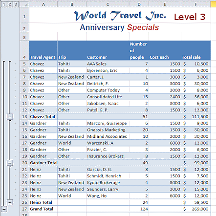
- Select A5:F23 on the Agent Totals sheet.
This is the data for all the travel agents but not the header row and not the Totals row. This selection creates a problem.
 On the Data tab in the Outline tab group, click on the button Subtotal
  .
.
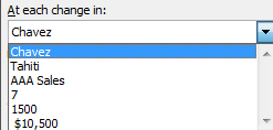
The Subtotal dialog appears.- Click the arrow to the right of Chavez to open the list
of choices.
These would be easier to understand if they were the column labels instead of the first data item in the column. - Click on Cancel to close the
dialog.
-
 Reselect the data and include the header row, A4:F23.
 - Click on the Subtotal button again.
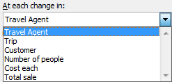
This dialog looks better! - Drop the list for 'At each change in:'.
This time we see the column labels. Much easier to understand! - Match your dialog to the one illustrated.
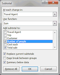
- Travel Agent.
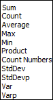
This is sets the group that you want to subtotal, for each different agent. That's why you had to sort first. - Sum
You can also use a function like Average or Max or Min or Count. It's odd to call these 'subtotals'! - Both Number of people and Total sale.
These will be the columns for which Excel will do a SUM subtotal. - Summary below data
This adds a Grand Total row.The Replace current subtotals box does not really matter this time, since there not any subtotals yet. If you Subtotal again later, you need the replace the old subtotals with the current ones.
- Travel Agent.
-
Click on OK to close the Subtotal dialog and apply your choices.
Look at what happens to the total you already had on the sheet. It's HUGE. This cell's formula adds up the column so it is adding the subtotals and grand total to what you really wanted. Whoops.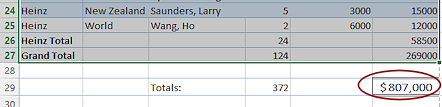
- Delete the row containing your original Totals, row 29.
- Save.
[trips22-Lastname-Firstname.xlsx]
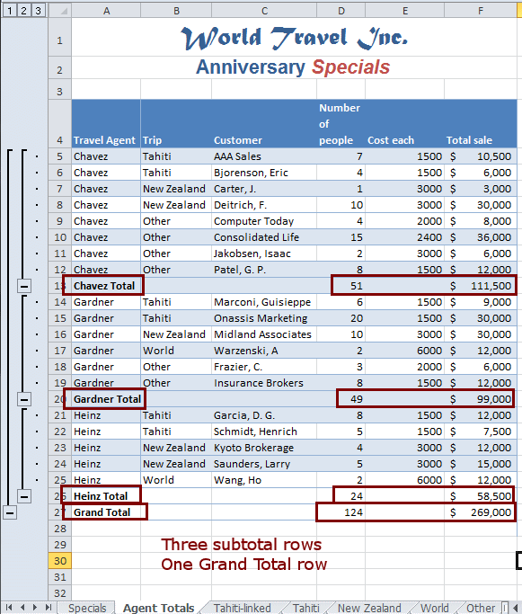
Your new subtotal and grand total rows inherit their background color from the row above.
Subtotal: Expand/Collapse
On the left is a new area, showing the arrangement of subtotals, which ones are expanded and which ones are collapsed.
A Collapse button ![]() shows that the area is currently expanded to show the data and the subtotals. Clicking this button will collapse the
display, hiding the data in that part of the table and showing only the subtotal.
shows that the area is currently expanded to show the data and the subtotals. Clicking this button will collapse the
display, hiding the data in that part of the table and showing only the subtotal.
An Expand button ![]() shows that the area is collapsed, showing only the subtotals. Clicking the button will
expand the display to show the rows of data also.
shows that the area is collapsed, showing only the subtotals. Clicking the button will
expand the display to show the rows of data also.
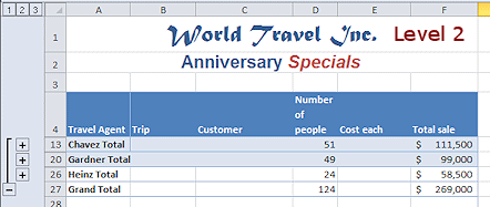
The number buttons ![]() at the top of this new area collapse and expand whole levels of the
display all at once-
at the top of this new area collapse and expand whole levels of the
display all at once- ![]() Level 1 = Grand Total,
Level 1 = Grand Total, ![]() Level 2 = all Subtotals,
Level 2 = all Subtotals, ![]() Level 3 = All Data.
Level 3 = All Data.
-
 Experiment: Expand/Collapse
Click on each of the buttons to expand and collapse the levels. Try different orders to your
clicks. Look at the row headings. Numbers come and go as you expand and
collapse. Notice what happens with the alternating row colors.
buttons to expand and collapse the levels. Try different orders to your
clicks. Look at the row headings. Numbers come and go as you expand and
collapse. Notice what happens with the alternating row colors.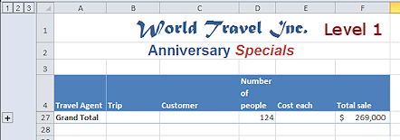
When you are ready to continue...
- Expand the whole sheet by clicking the Level 3 button, if necessary.
- Click on the
 and
and  buttons under Level 2 to expand and collapse individual sections of the
sheet.
buttons under Level 2 to expand and collapse individual sections of the
sheet. - Click the Level 2 button again, to show just the subtotals.
- Save.
[trips22-Lastname-Firstname.xlsx]
Repair Formatting: Borders Dialog
Adding in new lines and moving columns can mess up your formatting. Some borders are hard to see in Normal view, especially at the left edge of the sheet next to the window edge. The Borders tab of the Format Cells dialog lets you edit the borders for a single cell or for a selection, including the color and style for the border's line.
-
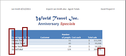 Look
at the Print Preview.
Look
at the Print Preview.
There are several glitches that are not easy to see in Normal view. (Your preview may look somewhat different.)
- Borders on Blank Row: The row
below the Grand Total should not have any borders.
How it happened: You deleted the original Totals row but not the blank row above it. The formatting for that blank row is hard to see in Normal view.
-
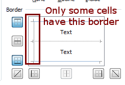
Borders on First Column: There should be a left border. There should not be a border between the first and second columns, which some cells have.
How it happened: You moved the Trip column to the right and it brought its left border with it. That left the Travel Agent column without a left border and with a border between the original cells in those two columns.
- Borders on Blank Row: The row
below the Grand Total should not have any borders.
- Select the row below the Grand Total and Clear Formats.
(Hint: Use the menu for the Clear button on the Home tab)
This removes the left and right border from the row but also the top border, which is also the bottom border for the Grand Totals. So the fix for one problem created another one. It's easy to fix! 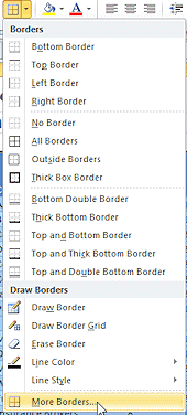 Select all of the rows from the header (row 4) through the Grand Total (row
27).
Select all of the rows from the header (row 4) through the Grand Total (row
27).
- On the Home tab click the arrow for the Border button to
open its menu.
You don't want to use one of the border choices on the menu. Those will apply the default line color Black. The border from the table style is blue. You need to open the full dialog.
-
 Select More Borders...
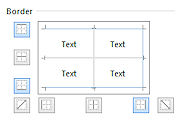
The Format Cells dialog opens to the Border tab.The preview in this dialog shows a solid border where all cells in the selection have that border and a fuzzy gray border where only some cells in the selection have that border.
Currently the selection does not have a left border.
-
Experiment: Borders
 Click various of the buttons surrounding the borders preview to create various combinations of
borders.
Click various of the buttons surrounding the borders preview to create various combinations of
borders.
These buttons are toggle buttons. Click to turn border on and click it again to turn border off.- Click directly on a border in the preview section to add and remove borders.
Select a different line style or color.
The preview does not automatically update! You must click on a button or on a border in the preview to apply this new choice.When you are ready to continue...
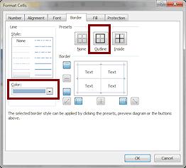 Set the line style to a thin solid line and
the color to Blue, Accent 1, Lighter 40%.
Set the line style to a thin solid line and
the color to Blue, Accent 1, Lighter 40%.
- Click on the button Outline to set a border around the
outside of the selection.
 Apply border to the horizontal middle line and remove border from the vertical middle line.
 Fuzzy gray borders: If there is a fuzzy gray border, it takes two clicks to remove the border. The first click applies a border and the second removes it.
 - Click on OK to close the dialog and apply your changes.
- Open Print Preview again.
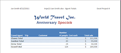
Compare your print preview to the image below. You should have a border around the whole table and horizontal borders for each row of data. If necessary, add any missing borders and remove any extra ones. - Save.
[trips22-Lastname-Firstname.xlsx]  Print just this sheet with only subtotals showing (Level 2).
|
|
| © 1997-2017 Jan Smith All Rights Reserved |
Site Map What's New |
Privacy Policy Terms of Service Copyright Acknowledgements |
~~ 1 Cor. 10:31 ...whatever you do, do it all for the glory of God. ~~
Last updated: March 22, 2017