Jan's Working with Numbers

Step-by-Step: AutoFill Data

Start with: trips4-Lastname-Firstname.xlsx (saved in previous lesson)

The special offer trips all have a fixed price. So there will be several duplications in the column labeled Cost Each. With AutoFill you don't have to type all of those separately.

Copy Cell Value: AutoFill

1. Save As  trips5-Lastname-Firstname.xlsx in your excel project2 folder.
2. In cell D5 type  1500  as the Cost Each for a Tahiti trip.

   You don't have to press ENTER for the next step to work.
   

   
3. Move the pointer over the lower right corner of cell D5 Until the mouse pointer changes to the Fill shape .
4. Drag downward to cell D10, in the last row with a Trip value of "Tahiti".

   Note the screen tip that shows what value you are copying.
   

5. Release the mouse button to complete the drag.

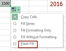
   The AutoFill Options button appears automatically whenever you drag the AutoFill handle.

6. Move your mouse over the button to see the arrow that opens the menu.
   The default Copy Cells is what you want this time. Later you will use other options.
   

   Excel 2013, 2016: Additional menu option, Flash Fill, which is covered in the next lesson .
   
7. Click in D11 to close the menu and be ready for the next step.
8. Type  3000  in cell D11 as the Cost Each of the New Zealand trip.
9. Fill the Cost each for the rest of the New Zealand rows by dragging the fill handle of cell D11.
    

Copy Cell Value: Key Combo

1. Type 6000 in cell D16 as the Cost each of the World trip and press ENTER. Now cell D17 is the selected cell.

2. Use the key combo CTRL + ' = +  
   That's a quote mark ' on the same key as a double-quote mark ".
   This will copy into cell D17, the value above it in the column. This is a very useful trick.

   If the cell above has a formula in it, this key combo copies the formula. If you want to copy just the value but not the formula itself, use CTRL + SHIFT + ".
   (Holding the SHIFT key down means the symbol at the top of the key will be used.)
   

3. Press ENTER.
4. Type in the following values, in order, for the Cost each of the trips in the Other category (D18 through D23).

   2000
   2400
   2000
   1500
   3000
   1500

5. Save.
    [trips5-Lastname-Firstname.xlsx] 

AutoFill: Simple Sequence

World Travel's spreadsheet doesn't yet have a place that uses a series of values. You will add a section to the spreadsheet that does. This new part will show the number of trips sold and their total value for each week that the special offers were available.

1. Scroll down to blank row 27.
   (You may need to use the scroll arrow instead of the box)
2. Type the following in cells A27 through D27:

    Week   Date    # of People   Total 

3. In cell A28, underneath the label Week, type  1 .
   
4. Drag by the fill handle of cell A28 down to cell A35.
   Hmmm. The 1 was copied into each cell. Not what you need this time. You want to number the weeks that the special offers were available.
   
5. Click on the AutoFill Options button to open the menu and click on Fill Series.
   The numbers change to 1, 2, 3,... 8. That's what we want!
   
6.  Save.
    [trips5-Lastname-Firstname.xlsx] 
    

AutoFill: Patterned Sequence

Once you enter a date, the cell will remember the format it used. Suppose you first type the date and it uses the default format:   1-Jun . Then you decide you want to see the date as  June 1, 2010 . If you retype it with the new format, it may be displayed as  1-Jun-98  or back to  1-Jun  instead! Frustrating! To change the formatting of the date you must use the Format Cells dialog, discussed in the next project. You cannot just retype differently

1. In cell B28, underneath  Date , type  June 1  and press ENTER.
   
2. Select B28 again and drag cell B28's fill handle down to B35.
   Excel fills a series automatically but the series it uses counts up a single day at a time. This column needs to show a week at a time to match column A. You need to establish a pattern for Excel to read.
   
3. Undo.
   
4. In cell B29 type  June 8 , which is a week after June 1.
    
5. Now select both B28 and B29 and drag the fill handle of the selection down to cell B35.

   Aha! AutoFill increased the dates by a week at a time by using the two selected cells to define the pattern for the series. More complex patterns would need more cells filled in to define the pattern.

    Default Alignment in Cell: Notice that text is aligned on the left and numbers and dates are aligned on the right. This default applies to all numbers, including dates and times. If Excel does not recognize what you entered as a date, it will be lined up on the left.
   

6. Center range A27:B35 and Column C by selecting them and clicking the Center button.
   Now the labels and the numbers are lined up better.
   
7. Save
   [trips5-Lastname-Firstname.xlsx]