Jan's Working with Numbers
Excel Basics: AutoFill
It is entirely boring to type in the same data over and over. And it certainly is not interesting to number lines 1, 2, 3, ... or fill in months of the year or days of the week. Excel's AutoComplete and AutoFill features are just the thing to handle these repetitious actions!
Example: AutoFill a Series
![]() Click the image below to see how AutoFill works to fill a series of days of the week.
Click again to
stop the animation.
Click the image below to see how AutoFill works to fill a series of days of the week.
Click again to
stop the animation.
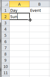
![]() AutoFill can fill in the
AutoFill can fill in the
days of the week for you.
AutoFill: Data
You use AutoFill to:
-
copy data to other cells in the row or column
- continue a pattern for data
 To use AutoFill, you just select a cell or cells and
hover over the bottom right corner of the selection until the mouse pointer
changes to the AutoFill shape, a black cross
 ![]() .
Drag the
fill handle over the cells you
want to fill - either down a column or across a row.
.
Drag the
fill handle over the cells you
want to fill - either down a column or across a row.
Examples:
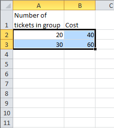
![]() Click the images below to see an animation of AutoFill at work. Click again to
stop the animation.
Click the images below to see an animation of AutoFill at work. Click again to
stop the animation.
| Copy Data: | Fill Series: |
 |
|
| |
|
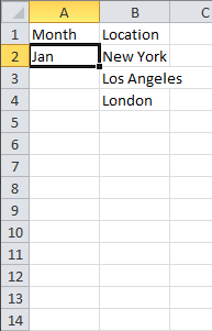
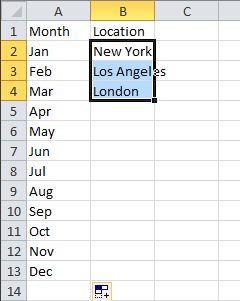
Excel can also work with patterns of words. If your sheet is a budget or a meeting calendar, for example, you will might list the months of the year. Once you have January typed in, AutoFill can complete the rest of the months for you. Pretty smart!
Excel also can fill the days of the week, quarters of the year, and any Custom List that you have created.
If you establish a pattern of any kind, Excel can repeat it down the column or across a row.
 |
 |
|
|
|
AutoFill: Formulas
AutoFill can also fill cells with formulas, adjusted for the new location. This is a blessing... most of the time. It's a problem if the formula uses a cell that should remain the same in all copies.
Some illustrations below were captured while formulas were showing. Column widths were adjusted to save space. When you switch back to showing values, you usually have to readjust the column widths.
![]()
![]() To show formulas on the sheet: CTRL + ` , which is the
grave accent key `, not the apostrophe '. On most keyboards it is to the left of the number keys.
To show formulas on the sheet: CTRL + ` , which is the
grave accent key `, not the apostrophe '. On most keyboards it is to the left of the number keys.
Example:
Formula uses cells all in the same column or row - Relative Cell References work
Download the example statistics.xlsx and click on the sheet tab Totals for the Year to follow along.
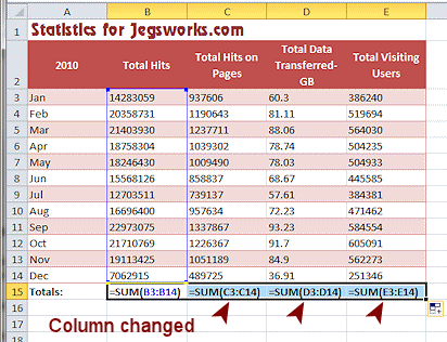 The formula in cell B15 adds up the values in the column
above it. The illustration shows the formulas created when you use AutoFill to copy the formula across the row into columns C, D, and E.
Excel
automatically changes the cell references to use the new column. Excel thinks of this formula as 'Add
up the values in the 12 cells above the formula's cell.'
![]() Formatting
copied: The formatting is automatically copied, too, unless you open the AutoFill
Options button
Formatting
copied: The formatting is automatically copied, too, unless you open the AutoFill
Options button ![]() at the bottom right of your copied cells and pick Fill
Without Formatting.
at the bottom right of your copied cells and pick Fill
Without Formatting.
Example:
Formula needs to use a fixed cell - Absolute Cell Reference needed.
You will run into trouble when you copy a formula that uses a value that appears only once on the sheet, like a total or the sales tax rate or an average for the year or the price of a ticket.
Download the example statistics.xlsx and look at the Percentages-Page Hits sheet to follow along.
The illustration show what happens when you use AutoFill to copy the formula =B3/B15 in C3 down the column. This formula is supposed to calculate a percentage, Hits in the month divided by the total for the year. The total for the year appears in cell B15.
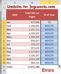
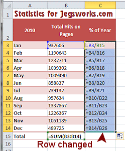
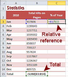
Problem = When you copy the formula down the column, Excel changes each cell reference to match the new row.
All the cell references are now for the same relative location, compared to the cell with the formula. 'Take the number that is one column to the left on the same row and divide it by the number that is 12 rows down and one column to the left'.
But the total we need is only in B15, not in B16 or B17, etc.! This results in
major errors -#DIV/0 -
because the formula is trying to divide by zero (a blank cell).
How to fix it: Absolute Reference
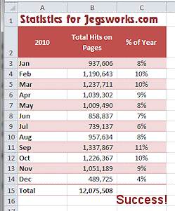
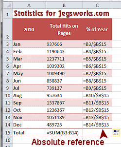 To
make the copied formulas use cell B15 every time, we must change the cell reference
from the relative reference B15 to an absolute reference $B$15. Then when we copy down the
column, the total for the year in B15 will be used. Success!
![]() Fill
without formatting: Formatting will be copied, too, making the
whole column match cell B3. After copying, open the AutoFill Options and
select Fill
Without Formatting. The original formatting reappears.
Fill
without formatting: Formatting will be copied, too, making the
whole column match cell B3. After copying, open the AutoFill Options and
select Fill
Without Formatting. The original formatting reappears.
![]() Absolute
Reference shortcut: F4 key on the keyboard rotates through all of the
choices
Absolute
Reference shortcut: F4 key on the keyboard rotates through all of the
choices
$B$15, $B15, B$15, B15. You can type in the $ if you wish, or when
you cannot remember what the key was!
For more on formulas, read the extra material on ![]() Formulas in the Appendix and do the
Formulas in the Appendix and do the ![]() review exercises.
review exercises.
Recalculation
Excel's Options can be set to automatically recalculate or to wait for you to tell it to recalculate after you make changes to formulas or to values used by formulas. The default is to automatically recalculate. It is easy to get in a panic when your formulas seem to be ignoring you because you forgot that you turned off automatic recalculation!
Make Excel Recalculate:
When something seems weird about the calculated values or when AutoFill seems to give wrong values, you can make Excel recalculate.
- Method 1:
 Press the F9 key to make Excel recalculate the
values.
-
 Method
2: Formulas tab > Calculation tab group > Calculate
Now for whole workbook or Calculate Sheet for
just the current sheet
How to change when Excel recalculates:
-
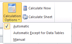 Method
1: Formulas tab > Calculation tag group > Calculation Options
-
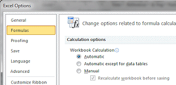 Method
2: Office button or File tab > Excel Options > Formulas >
Calculation Options
AutoComplete

After typing a C in cell F3,
Excel offers to complete the word.
Excel pays attention to what you have already entered in each column. When you start entering data in a new cell, Excel may offer to complete your typing for you. For example, if you are entering a list of names and addresses, it is likely that many of them will have the same city and state and even the same street. It can save a lot of typing if you let Excel finish out the ones that repeat.
To accept Excel's suggestion, just make another cell active by doing one of these actions:
-
Press ENTER
-
Press TAB
-
Press an arrow key
-
Click in a different cell
Note: Excel will not make a suggestion unless it sees only one matching choice in the list of things you have already typed in that column. If there are blank cells in the column, Excel will ignore the values above the blank.

