
Jan's Working with Numbers
Excel Basics: AutoFill: AutoSum
 The formula used the most is SUM. The AutoSum
feature makes it easy to total columns or rows. Excel will guess what
cells you want to add based on which cells are empty. A neat trick!
The formula used the most is SUM. The AutoSum
feature makes it easy to total columns or rows. Excel will guess what
cells you want to add based on which cells are empty. A neat trick!
AutoFill can help copy a formula across a row or down a column. Just be careful that all cells used in the formula are in the same row or same column.
If you need to use a fixed cell, you must use an absolute reference for that cell.
| |
Step-by-Step: AutoSum |
|
| What you will learn: | to enter data in a column |
Start with: ![]() trips6-Lastname-Firstname.xlsx (saved in previous lesson)
trips6-Lastname-Firstname.xlsx (saved in previous lesson)
Data Entry
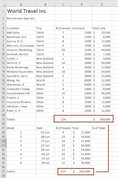
- Complete the table at the bottom of the sheet by filling in the values for # of people and Total as shown
here.
# of people Total
9 17000
23 36000
18 27000
18 36000
12 24000
20 51000
12 42000
12 36000
 Save As trips7-Lastname-Firstname.xlsx to
the excel project2 folder on your Class disk.
Save As trips7-Lastname-Firstname.xlsx to
the excel project2 folder on your Class disk.
AutoSum: Upper Table Totals
- Select cell A25 and type Totals:
- Select cell C25 and click
 the AutoSum button
on the Home tab.
the AutoSum button
on the Home tab.
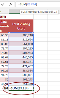
Excel guesses you want to add values in above, range C5:C24, and surrounds that range with a blinking dashed border. The formula looks like =SUM(C5:C24)The range includes a blank cell, which Excel understands and will ignore.
- Press ENTER to accept Excel's formula.
- Select cell E25 and click the AutoSum button.
- Press ENTER to accept the formula =SUM(E5:E24)
-
Save.
[trips7-Lastname-Firstname.xlsx]Why did we skip column D? That column shows the cost for one trip. The total of those numbers is not useful!
Type Formula
-
 Select cell A37 and type Totals:
 - Select cell C37 and type =sum(c28:c36
Notice that you did not have to use upper case letters but you must use the = and the parenthesis ( . - Click the check mark button on the Formula Bar to accept your formula.
The selection stays in the same cell so you can read the formula.
Excel adds the closing parenthesis for you.
This method works when Excel is confused about what to add.
AutoFill Formula: Lower Table Totals
-
 Autofill from cell
C37 to D37.
Autofill from cell
C37 to D37.
(Move the mouse pointer over the bottom right corner of C37 until it changes to the AutoFill shape and drag to the right.)
The formula in C37 is copied into D37 but the cell references are changed.
This method would be really helpful when there are a lot of columns that use the same type of formula.
- Click in cell D37 and look at what the Formula
Bar shows.
=SUM(D28:D36)(Check: are the totals in the lower table the same as in the upper table? They should be.)
- Save.
[trips7-Lastname-Firstname.xlsx]
Format Numbers: Accounting Style
Now that you have your totals for rows and for the Totals columns, it would be nice to have them look like money! The Home tab and Mini-Toolbar have a $ button that will apply the currency formatting from the Regional Settings in the Windows Control Panel.
-
 In
the Name box, type the following: E5:E23, E25, D28:D35, D37 and press the ENTER key.
In
the Name box, type the following: E5:E23, E25, D28:D35, D37 and press the ENTER key.
All cells and ranges listed are selected at once. Sweet! - Click
 the Accounting Style button.
Each selected cell is formatted as money, $ and two decimal places. - Click
 the Decrease Decimals button twice to remove zeros.
None of the values have any cents so the zeros don't help. - Save.
[trips7-Lastname-Firstname.xlsx]
Formula with Absolute Reference
Next you are going to add some formulas to create a new column on the lower table. The cells will calculate what percentage of the total sales each week contributed. You will see exactly what can happen when you autofill a formula that needs a value that is in only one cell and how to fix that problem.
-
 Click in cell E27 and type % of Total and press ENTER.
The label text is accepted and the selection moves down to cell E28. - In cell E28 enter the formula =d28/d37 and click the
check mark button
 on the Formula bar.
The formula is accepted but the selection stays in cell E28.
The calculation produces a long decimal value.
-
 Drag the AutoFill handle for cell E28 down the column
to cell E35.
Drag the AutoFill handle for cell E28 down the column
to cell E35.
There is an error code in all the cells below E28, #DIV/0!
This code means that the value that the formula tried to divide by was zero or was text.
-
Click in cell E29 and inspect the formula in the Formula Bar.
AutoFill changed the row part of the cell references for the numerator and the denominator to =D29/D38
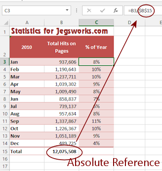
But cell D38 is empty.You need to modify the original formula to use an absolute reference for the total in D37, which will not change when the formula is copied.
-
 Double-click on cell E28.
Edit mode turns on.
- Click in the cell to the right of D37.
- Press the F4 key on the
keyboard once.
(F4 is on the row above the number keys on most keyboards.)
D37 turns into $D$37, which is the form for an absolute reference that will keep AutoFill from changing this part of the formula.
- Click the
check mark button on the Formula bar.
-
 Drag the AutoFill handle for cell E28 down to E35 again.
Now we see lovely decimals!
- Save.
[trips7-Lastname-Firstname.xlsx]
Format Numbers: Percent Style
-
 While
the E28:E35 is still selected, right click the
selection.
While
the E28:E35 is still selected, right click the
selection.
The Mini-Toolbar appears along with a menu.
- From the Mini-Toolbar, click on the Percent
Style button
 .
.
The values change to the default style for percentages, with no decimals.
- Save.
[trips7-Lastname-Firstname.xlsx]
Show Formulas
You must check your work by checking the formulas, not just the values in Normal view.
-
 Show formulas, CTRL + `
- Hide formulas again with the same key combo.
|
|
| © 1997-2017 Jan Smith All Rights Reserved |
Site Map What's New |
Privacy Policy Terms of Service Copyright Acknowledgements |
~~ 1 Cor. 10:31 ...whatever you do, do it all for the glory of God. ~~
Last updated: March 22, 2017