Jan's Working with Numbers

Step-by-Step: Print with the Defaults

Start with: , trips8-Lastname-Firstname.xlsx (saved in previous lesson)

Print: Defaults

1. Save As  trips9-Lastname-Firstname.xlsx  to your Class disk in the excel project2 folder.
2. Click on the tab for Sheet1 to make it the active sheet.
   If cells are selected, click on a blank cell to remove the selection.

3. Switch  to the Review tab and click on Spell Check .

   Excel checks spelling down the document from the current cell. If the current cell is not A1, you will see a message asking if you want to continue checking spelling from the beginning of the document. Usually you would want Excel to check the whole document.

4. Click Yes.

   Many of the names in the Customer column will be unknown to Excel's dictionary. Look carefully to see if you've typed the name in correctly. Do not add these names to the dictionary.

5. Open the Page Setup dialog:
   Page Layout tab > Page Setup dialog box launcher .
   Inspect all tabs and make corrections to the settings if necessary.

   Page - Portrait, 100%, Letter size

   Margins - top and bottom 1 inch, left and right 0.75 inch, header and footer 0.5 inch

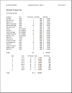
   Header - Create a Custom Header with your name and date, file name - sheet name, Excel Project 2

   Sheet - all text boxes blank.  Page order: Down then over.
   

6. Click OK to close Page Setup.
    
7. On the Status bar click on the button for
   Page Break Preview .

   The whole sheet fits neatly on one page.
    
   If the wide blue line leaves some cells with data outside, drag the lines to include the cells. If Excel refuses to include all cells, adjust the width of your columns.
   

8. Open Print Preview and check that all looks right:
   
   Excel 2007: Office button > Print > Print Preview
   
   
   Excel 2010, 2013, 2016:
   File tab > Print 
9. Print with the default settings:.
   
   Excel 2007: Print button on the Print Preview ribbon and then OK.
    
   
   
   Excel 2010, 2013, 2016: Print button to the upper left of the preview and then OK.
   Only the active sheet prints.
10. Save
     [trips9-Lastname-Firstname.xlsx]  
    

Add Button to Quick Access Toolbar

Are you tired of needing multiple clicks to get to Print Preview. You can add a button to the Quick Access Toolbar to go straight to it!

1. At the top of the window, click the More button at the right end of the Quick Access Toolbar.
   
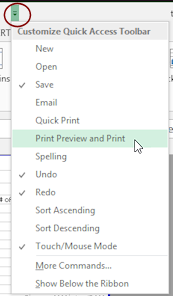
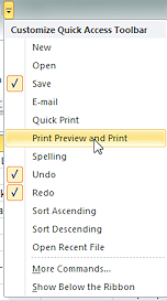   A list of buttons that are often added to the toolbar appears.
   A check mark by a name means that button is already on the toolbar.

   The default buttons are Save, Undo, and Redo (which changes to the Repeat icon when the action can be repeated in a different spot.

2. Click on Print Preview or Print Preview and Print.
   
   A new icon appears at the right end of the toolbar.

   

Print: Chart Sheet

1. Click on the tab Pie Chart - people to make it the active sheet. 

2. If necessary, click on the chart to select it.
   There are resizing handles on the chart
   Handles are gray dots or circles on the chart border in the corners and middle of each side.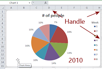

   

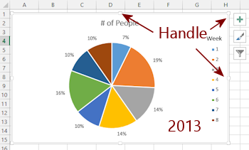
   The Name Box shows "Chart 1". If you created the chart more than once, the number after 'Chart' will be larger than 1 even if you deleted those other versions of the chart.
   

3. Open Print Preview with the new icon on the Quick Access Toolbar.
   All you see is the chart stretching across the whole width of the page. None of the cells on the sheet show. How unexpected!

   Printing when chart is selected: If a chart is selected, Excel will print only the chart itself AND will make it as large as possible.
   

4. Return to Normal view.
   
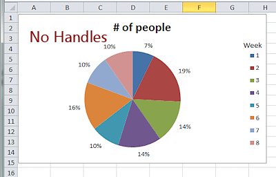5. Deselect the chart by clicking on a cell outside the chart.
   No border and no handles should be showing around the chart.
   The Name Box shows the cell reference where you clicked.
    

6. Open Print Preview.
   Now the chart is in the upper left of the page. Much smaller.

   But, there is no header showing! You must set the header separately for each sheet in a workbook or else group the sheets and then set the header. <sigh> 

7. Open Page Setup while still in Print Preview.

   Excel 2007: Page Setup button on Print Preview ribbon
   Excel 2010, 2013, 2016: Click the link Page Setup in the lower left of the preview.
   The Page Setup dialog opens.
   
8. Click on the Header/Footer tab and create a custom header with your name, two spaces, the date in the Left section, File name - Sheet name in the Center section, and Excel Project 2 in the Right section.
9. Click on OK to close Page Setup.
    
10. Click the Print button in the Print Preview window.
    The Print dialog opens. Use the default settings to print the active window.
    
11. Click OK to print the chart sheet. 
12. Save
     [trips9-Lastname-Firstname.xlsx]