Jan's Working with Numbers

Step-by-Step: Insert

---

What you will learn:

to insert a column to insert a row to insert a cell to fix formatting issues to delete cells to insert a sheet to reorder sheet tabs

---

Start with: trips16-Lastname-Firstname.xlsx - Sheet1 (saved in previous lesson)

You will now insert a column for the name of the travel agent who arranged each special offer trip. You will adjust the spacing in the sheet by adding a row, though it might be more efficient to resize the blank row that is already there.

A little experimentation will show you that adding a cell or two in the middle of things is not often a good idea.

You will add several sheets to the workbook, which you will use later to show information about each special trip separately.

---

Insert: Column

You've decided that you want to include the name of the travel agent in charge of each trip. You need to add a column to the upper table.

1. If necessary, open trips16-Lastname-Firstname.xlsx from your Class disk.
   
2. Save As trips17-Lastname-Firstname.xlsx in the excel project3 folder of your Class disk.
   
3. Click on the tab for Sheet1 to make it the active sheet..
4. Select all of Column B.

5. On the Home tab in the Cells tab group, click the Insert button (not its arrow).
   A new column appears to the left of the selected column.

   The new column uses the same background formatting as the existing columns..
   The new column cells in rows 1 and 2 are included in the merged cells for the title and subtitle. 

6. Select cell B4 and type  Travel Agent  and press ENTER.
   Your typing is formatted like all the other labels. Hurrah!!
7. Type in the names for the three travel agents responsible for the special offer trips, as shown in the illustration at the right.

   AutoComplete: Once you have entered a name the first time in a column and then start typing that name in another cell in the same column, Excel will offer to AutoComplete your typing. Excel displays its suggestion as highlighted in the cell, like the final entry in the illustration. Press ENTER or press the down arrow to accept the offer and to move the selection down a cell. This will save you a lot of typing!!
   

8. Save.
   [trips17-Lastname-Firstname.xlsx]
    

---

Insert: Row

You decided that you need more space between the upper and lower tables on Sheet1. You could change the height of Row 24 but you decide to insert another row. We are practicing still!

1. Select cell C27.
   
2. On the Home tab in the Cells tab group, click on the Insert button (not on its arrow).
   Whoops. Only a single cell was inserted, which moved the cells below down.

   Why?

   The Insert button looks at what is currently selected and inserts a blank one of those. Previously you had a whole column selected, so Excel inserted a whole column. This time you had selected only a single cell, so Excel inserted just one cell. This is not often something you want to do!

3. Undo.
   

4. Click the arrow on the Insert button.
   A menu of choices of what to insert appears - Cells, Rows, Columns, Sheet.

   However many rows or columns or cells are selected in how many will be inserted.
   

5. Click on Insert Sheet Rows.
   A blank row is inserted above the current row.
6. Save.
   [trips17-Lastname-Firstname.xlsx]
   

---

Insert: Cell

Inserting cells requires that something be moved to make room. Like in the last lesson when you moved data, you only have the choices to move data right or down, but not both at the same time.

1. Select cell D25, the total number of people.
2. Right click on the selected cell.
   The context menu appears.

3. Click on Insert...
   The Insert dialog appears.

   You have four choices. Notice that you can insert a whole row or column with this method.
   
   

4. Verify that Shift cells down is selected and click on OK.
   Hmmm. The contents of D25 and the cells below shift down one row, along with their formatting.
   

   This effect could be useful if you find you have entered some data in the wrong rows or columns. However, it would be easy to scramble a table by inserting a cell or two without careful thought.

5. Since this is not very useful at this point, Undo.

   Let's use the same method to insert a whole row.
   

6. Select cell D25, right click on the selection, click on Insert..., click on Entire row and then click on OK.
   
   A blank row is inserted above the row with your totals, moving what was row 25 and the rows below it down one row.

   Did you notice that the inserted row inherited the formatting of the row above, not the row that was selected. Did you expect that?  
   

---

Fix Formatting: Reapply Table Style

When you move or insert new rows, columns, or cells after you have done cell formatting, you often find that your formatting needs to be repaired.  

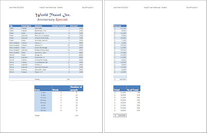
1. Open Print Preview.

2. Inspect the print preview.
   Formatting glitches show in the preview that were hard to notice in Normal view.
   The borders for the upper table are inconsistent. Borders are missing in some spots and appearing where they don't really need to be.

   These borders came from the table style. Originally there was a border around the outside of the table and a border between rows.

   Moving columns and inserting a row and disturbed the pattern!

   In Normal view it is hard to see whether or not the cells in column A have a left border. Only Print Preview makes this clear.

   The easy way to fix this table is to reapply the table style... but you must remember to clear formatting at the same time.

3. Select the upper table, A4:F26
   
4. On the Home tab, click on Format as Table to open the gallery of styles.
   
5. Right click on Medium 2 and then click on Apply and Clear Formatting.
    
   
6. Click on OK in the Format as Table dialog.
   The selection becomes a 'table' with a sorting arrow for each column.
   
7. On the tab Tables Tools: Design, click on the button Convert to Range .
   
8. Click on Yes in the message box that asks, Do you want to convert the table to a normal range?
   The selection is back to a normal range.
9. If necessary, fix any other formatting problems, like missing Currency format.
   

---

Check Print Preview 

1. If necessary, on the Page Layout tab in the Scale to Fit tab group, set Scaling to 100%.
   (In a previous lesson you may have set scaling to '1 page'. Don't you just love breaking things on purpose so you can fix them?!)
   
2. Open Print Preview.
   Are the formatting problems fixed? Yes... and No!
   • The borders look good - that's the 'Yes' part.
   • 'Number of people' does not wrap because of how wide the column is.
   • The total in cell F26 lost its cell style.
   • The sheet may be taking more than one page! That is likely from the columns widths being too wide to fit on one page.<sigh>
     (Your results may vary, depending on the exact widths of your column and your page margins.)
      
      Fixing one problem can create or reveal others! We can handle this... with some work.
     

   

3. Save.
   [trips17-Lastname-Firstname.xlsx]

---

Fix Formatting

Row 25 is not doing anything important. Let's get rid of those cells! Then maybe we can fix the issues that our 'fix' created.

1. Select A25:G25.
   We need to catch the cell above the last column in the bottom table, too.
   
2. On the Home tab in the Cells tab group, click the Delete button.
   The cells are deleted and all cells below the selection move up.
   
3. Save.
   [trips17-Lastname-Firstname.xlsx]
   

---

Fix Formatting

What formatting issues need to be fixed? The column widths and cell style for the total. Let's fix them all! Those columns widths will take the most steps.

1. Select column D.
   
2. Resize the column width to 60 pixels, or 7.86 characters
   This is just wide enough for the word Number in cell D4.
   Part of the column label in cell D4 is still hidden. You need to make the row taller.
   
3. AutoFit row 4.
   It will be 60 pixels high.
   A dotted page break line will show if the sheet will still take two pages.
   More adjustments!
   Next you will adjust column B to be just wide enough for the travel agents' names.  
   
4. Drag the right edge of the header for column B to just fit the longest travel agent name, Gardner.
   (That is about 56 pixels wide.)
   The column label, Travel Agent, is cut off.
   
5. Click in cell B4.
   

6. On the Home tab in the Alignment tab group, click on the Wrap Text button .
   The text in the cell wraps to two lines. The row height is already tall enough. Yeah!

   Is the sheet onto one page yet? Maybe... or perhaps not yet. The percentages in column G in the lower table may not fit yet.
   There are several ways to tell.

   How to check the number of pages

   • Open Print Preview and look at the number of pages.
   • Switch to Page Layout view and check which pages have cell content.
   • Switch to Page Break Preview and see where the dotted lines fall.
   • Look at the Normal view for a dotted line (if you already looked at Print Preview in this work session.)
     

   You could shift that lower table to the left one column, but that messes up the text wrapping for 'Number of people' in row 28.
   Let's try one more column width change.

7. AutoFit column F.
   The dotted line in Normal view should show that we have success!
   All cells fit onto one page when printing!!

   One more formatting fix.
   

8. Click in cell F25, the total of sales.
   

9. On the Home tab in the Styles tab group, click on the custom cell style Totals.

   Finally! All the formatting messes caused by inserting and moving cells are cleaned up.
   Just remember in the future - format last! If you change your mind after creating lovely formatting, you will just have to deal with the mess your created! You can handle it!
   

10. Save.
    [trips17-Lastname-Firstname.xlsx]

---

Insert Sheet and Reorder Sheet Tabs

You need to create some new sheets to which you can copy data in the next lesson. You currently have three sheets including the sheet Tickets Sold Chart.

1. On the Home tab, click the arrow by the Insert button.
2. Click on Insert Sheet.
   
   A blank sheet tab appears, named Sheet2.
   (Your sheets will have different numbers if you have inserted and deleted sheets already. That is not a problem!)

   A new sheet always appears to the left of the active sheet with this method.

3. Repeat to insert 2 additional sheets, Sheet4 and Sheet5.  
4. Rename Sheet1 (the one that you have been working with) as Specials and drag it to the far left of the sheets tabs.
5. Rename another sheet as Tahiti and drag it to the right of Specials.  
   The small black arrow shows where the sheet will be placed when you drop it.
6. Rename other sheets as New Zealand, World, and Other.
7. Save.
   [trips17-Lastname-Firstname.xlsx]