
Jan's Working with Numbers
Format: Arrange: Link
Excel makes it easy to enter data once and then have it show up in different places or on different sheets. Quite a time-saver. And it reduces the chances for error.
Linking cells makes a copy that changes whenever the original changes.
Paste Link in the Paste Special dialog or Paste icons will let you create this kind of data link for multiple cells at a time.
You can also link single cells by typing in the cell reference including the sheet name in the form =sheetname!cellreference, like =Specials!D4 . Note the ! exclamation point between the sheet name and the cell reference or name. When reading this formula aloud, you say 'bang' for the exclamation point, like "equals Specials bang D four".
| |
Step-by-Step: Link |
|
| What you will learn: | to create a link by typing the cell reference to create a link by clicking the cell to insert a new sheet using the ribbon to use Paste Link to use Format Painter on linked cells to correct formatting and formula errors and remove unneeded zeros to print the sheet showing the links (formulas) |
Start with: ![]() trips18-Lastname-Firstname.xlsx
(saved in previous lesson)
trips18-Lastname-Firstname.xlsx
(saved in previous lesson)
To have the data on the sheet Tahiti updated whenever the original on the sheet Specials changes, you must link the cells.
In the Formula bar =Specials!A4 would link that cell to cell A4 on the Specials sheet. Note the exclamation point ! between the sheet name and the cell reference. You can do this yourself if there are just a few cells. To do this for many cells at once you can use Paste Link on the Paste Special dialog or use the Paste Link icon in Excel 2010, 2013, and 2016 to link them when you paste.
When you link cells, you do not get the formatting also. You must apply the formatting separately.
Create Link: Keyboard
-
 Save
As trips19-Lastname-Firstname.xlsx in the excel project3 folder of
your Class disk.
Save
As trips19-Lastname-Firstname.xlsx in the excel project3 folder of
your Class disk. - Select cell A1 on the sheet Tahiti.
-
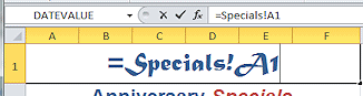 Type =Specials!A1 and click
  the
check mark button on the Formula bar.
the
check mark button on the Formula bar.
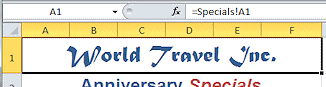 The
cell A1 is still selected and looks the same as before, but now, if
you change cell A1 on the sheet Specials, this cell will
change, too. This is the purpose of linking.
The
cell A1 is still selected and looks the same as before, but now, if
you change cell A1 on the sheet Specials, this cell will
change, too. This is the purpose of linking.
- Save.
[trips19-Lastname-Firstname.xlsx]
-
 Experiment: Test Linking
Switch to the sheet Specials and edit cell A1 in some way.
Return to Tahiti to see if its cell A1 changed to match.
(It should have!)Use Undo to return cell A1 remove your changes.
(You do not have change sheets first. There is only one Undo list.)
Create Link: Mouse
You can click with your mouse to link cells. This method avoids the problem of fumble fingers not typing the name of the sheet or the cell reference correctly. When you have a lot of cells to link, it gets tiresome to type the reference for every cell in the table.
-
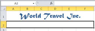 Select cell A2 on sheet Tahiti.
 -
Right click on the selection and choose Clear Contents.
The cell is now blank but it is still merged.Alternate method: Home tab > Clear button> Clear contents
-
 Type an equals sign =
 - Switch to sheet Specials and click on cell A2.
- Press ENTER.
You are switched back to the sheet Tahiti automatically.
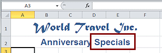
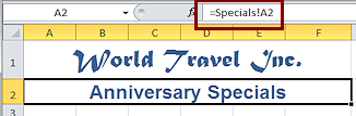
The text 'Anniversary Specials' shows up, but your manual formatting for the word 'Specials' is missing. -
 Select cell A2 again.
The Formula bar shows = Specials!A2 for the contents of cell A2. You cannot edit here to format just part of the text when the text is linked.
- Save.
[trips19-Lastname-Firstname.xlsx]
Next we will look at a method for linking cells and getting the same formatting.
![]() Finish your linking! If you
forget to press ENTER after selecting the cell to link, your next clicks also put cell references in the Formula bar. Quite a mess! The
Undo command is a real help when this happens.
Finish your linking! If you
forget to press ENTER after selecting the cell to link, your next clicks also put cell references in the Formula bar. Quite a mess! The
Undo command is a real help when this happens.
Add a New Sheet
To learn how to Paste Link we could delete all of our Tahiti work, but instead let's create a new sheet to work with.
-
 If
necessary, make the Tahiti sheet the active sheet.
If
necessary, make the Tahiti sheet the active sheet.
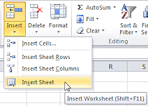
- On the Home tab, click the arrow for the Insert button to open its list.
-
 Click on Insert Sheet.
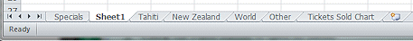
A new blank sheet appears, listed between Specials and Tahiti. The number of the sheet will depend on whether or not you have closed and reopened the workbook along the way.
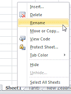 Right
click on the sheet tab for the new sheet and click on Rename.
Right
click on the sheet tab for the new sheet and click on Rename.
- Type as the new name Tahiti-linked and press the ENTER key.

Link: Paste Link
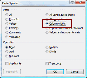
Using Paste Link to link a number of cells will not copy the formatting of the original cells or the column widths. But, as you learned in the last lesson, you can repeat your paste with different choices. Since you must paste the column widths first in Excel 2007, the steps below will do that for all three versions. Just be careful not to 'do' anything before you finish your pasting or you will have to copy again.
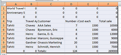
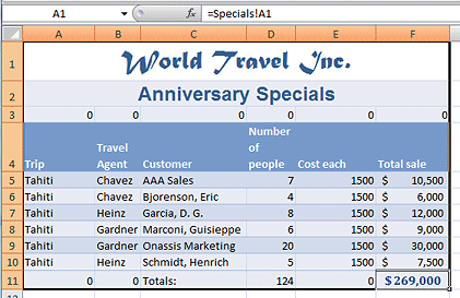
 Switch to sheet Specials and select ranges A1:F10 and A25:F25 (the data about Tahiti trips) again
and Copy.
Switch to sheet Specials and select ranges A1:F10 and A25:F25 (the data about Tahiti trips) again
and Copy. - Switch to sheet Tahiti-linked and select cell A1.
- Click the Paste button to open its menu.
- Click on Paste Special..., and then on Column Widths.
No data is pasted yet.
-
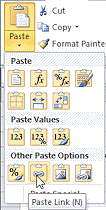
 Click on Paste and then click on Paste Link
 .
.
(The icon shows links in a chain.)
The non-adjacent data you copied is pasted on the sheet Tahiti as adjacent cells. The cell widths remain. Hurrah!All the cells in the table on Tahiti-linked are linked to the cells in Specials.
-
 Click on several cells and check that the Formula Bar shows the link.
Problems that remain after using Paste Link:
- No formatting was copied.
- A zero appears if the original
cell was blank.
All of these problems are fixable.
Fix Formatting
Our previous trick of pasting again with a different type of pasting may help out again.
Fix Problem (a): Formatting
-
 Switch to sheet Specials and, if necessary, select ranges A1:F10 and A25:F25 (the data about Tahiti trips) again.
(If the blinking border is still on, you don't have to select again.)
- On the Home tab in the Clipboard tab group, click the Format Painter button

 .
.
- Switch to the sheet Tahiti-linked and click cell A1.
All cells are formatted like they were on Specials. It's magic! - Click in several cells to be sure that the links are still there. They certainly should be.
Alternate methods: Paste Formatting
- Paste Special dialog > Formats
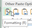


 Excel 2010, 2013, 2016: Paste button > Formatting icon

 Notice the
(R) in the screen tip for this icon. That means that once this
palette of icons is displayed, you can press the R key to
execute the command when the palette of choice is open.
Notice the
(R) in the screen tip for this icon. That means that once this
palette of icons is displayed, you can press the R key to
execute the command when the palette of choice is open.
Fix Problem (b): Zeros instead of blank cells
-
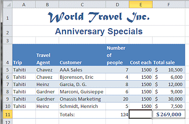 For
each cell with a zero in it, select the cell and press the
DELETE key.
For
each cell with a zero in it, select the cell and press the
DELETE key.
That's all of row 3 and A11, B11, E11,
- Save.
[trips19-Lastname-Firstname.xlsx]
Repair a Formula
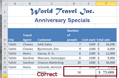
Something odd is going on with the totals cells. These totals cells show the sums for the whole column on the sheet Specials. This is not what you really want. You want the sum of the values that are on this sheet. So these totals cells should not be linked after all.
-
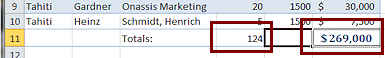 Select cell D11 and click on the AutoSum button and press ENTER.
 - Repeat for cell F11.
-
 Save.
Save.
[trips19-Lastname-Firstname.xlsx]
Test the links
-
Experiment: Test the links
Change some values for the Tahiti trips on the Specials sheet, and then look at the Tahiti sheet to see if the changes are shown there.
Change the names as well as the number of people and the price per ticket.Undo all your experiments!
(Remember- You saved before you started your experiments. You can close the file without saving changes and open it up again to get back to where you were.)
Sheet Header
- With sheet Tahiti-linked active, open Print Preview.
There is no header! Sadly, you must make an effort to create a header for each sheet in a workbook. You CAN select several sheets at once and create a header that will apply to all of them. -
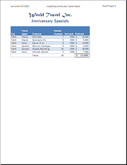 Click on the Page Setup and then the Header/Footer tab.
 - Create a custom header for the Tahiti-linked sheet - Left section has your name and the date; Center section has the file name and sheet name; Right section has Excel Project 3. Click OK to close the dialog.
- Make corrections to the sheet if necessary.
-
 Print.
 - Save.
[trips19-Lastname-Firstname.xlsx]
Print Showing Links
When things go wrong, it might be easier to proof a printed page instead of looking at the computer screen. You can print a copy that shows the links, which are just a type of formula.
- With
the sheet Tahiti-linked active, use the key combo CTRL + ` to show
formulas.
(That ` symbol is the accent key that is usually to the left of the number 1 key on English keyboards.) -
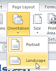 On the Page Layout tab, use the Orientation button to change the orientation to Landscape.
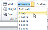
- On the Page Layout tab in the Scaling tab group, set Width to 1 page.
-
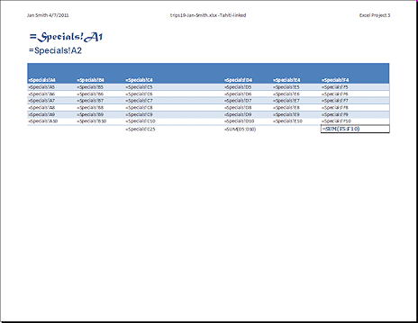 Open Print Preview and verify that all is going to print
correctly.
Open Print Preview and verify that all is going to print
correctly.
- Print.
- Switch back to normal display with the key combo CTRL + `
- Save.
[trips19-Lastname-Firstname.xlsx]
|
|
| © 1997-2017 Jan Smith All Rights Reserved |
Site Map What's New |
Privacy Policy Terms of Service Copyright Acknowledgements |
~~ 1 Cor. 10:31 ...whatever you do, do it all for the glory of God. ~~
Last updated: March 22, 2017