
Jan's Working with Numbers
Formulas: Images: AutoShape
An AutoShape is a drawing object that Excel has already designed for you. There a many of these AutoShapes and you can group them into even more complex drawings.
![]()
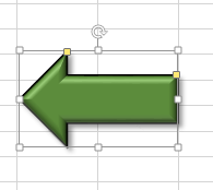
 Once
you select a shape from the palette, you can click in the document to create
a shape with the default size and color (blue). Or you can drag in the
document to create a shape of whatever size you want. Of course you can
resize a shape afterwards and format it with a different fill or border or
effect. Many shapes have one or more yellow adjustment handles that you can
drag to adjust features of the shape.
Once
you select a shape from the palette, you can click in the document to create
a shape with the default size and color (blue). Or you can drag in the
document to create a shape of whatever size you want. Of course you can
resize a shape afterwards and format it with a different fill or border or
effect. Many shapes have one or more yellow adjustment handles that you can
drag to adjust features of the shape.
| Handle: | Changes: | |
|---|---|---|
| Resize handle in a corner. | Both length and width at once. Proportions can change as you drag a corner! |
|
| Resize handle in middle of edge | Only one dimension - either length or width | |
| Rotation handle | Rotates the whole shape. | |
| Adjustment handle | Changes the size, proportions, or location of parts of the shape. | |
| |
Step-by-Step: Add AutoShape |
|
| What you will learn: | to show/hide AutoCalculate functions on the Status Bar to use AutoCalculate to insert an AutoShape to format an AutoShape to copy and paste an AutoShape to delete an AutoShape that shapes are attached to cells but are not in the cells |
Start with: ![]() trips23-pivottable-Lastname-Firstname.xlsx - Formatted Groups sheet (saved in previous lesson)
trips23-pivottable-Lastname-Firstname.xlsx - Formatted Groups sheet (saved in previous lesson)
 On
the Status bar there is a wide space to the left of the Views buttons that shows values that
are calculated
whenever you select cells with numbers in them. The default is to show the Average, Count, and Sum. You can
right click on the Status bar to select which functions you want to see in
this AutoCalculate area. To take
advantage of this feature, all you have to do is remember that it is there!
On
the Status bar there is a wide space to the left of the Views buttons that shows values that
are calculated
whenever you select cells with numbers in them. The default is to show the Average, Count, and Sum. You can
right click on the Status bar to select which functions you want to see in
this AutoCalculate area. To take
advantage of this feature, all you have to do is remember that it is there!
You are going to add a shape to draw attention to the maximum Totals in the upper and lower tables. First you need to find out which cells have the maximum values. Excel's AutoCalculate feature will help, especially when there are many values to inspect.
AutoCalculate
-
 Open trips23-pivottable-Lastname-Firstname.xlsx to
the Agent Totals sheet.
Open trips23-pivottable-Lastname-Firstname.xlsx to
the Agent Totals sheet.
- Save
As trips24-Lastname-Firstname.xlsx in the excel project4 folder of your Class
disk.
-
 Switch, if necessary, to the sheet Formatted Groups.
- Right click on the Status bar to open the context menu.
Find the section with Average, Count, and Sum, which should be checked. - Click on Maximum, which
shows the Maximum value in whatever you have selected.
-
 Select all of the Total Sale values, F5:F23.
- Inspect the Status Bar.
It shows the largest of the values selected. Unhappily, Excel does not tell you which cell contains the maximum. - Find the cell contains the Maximum and make note of its cell reference.
You are going to insert an AutoShape to point out this cell. - Save.
[trips24-Lastname-Firstname.xlsx]
 Experiment:
AutoCalculations
Experiment:
AutoCalculations
- Make different selections and look at how the Status bar updates.
- Open the right click menu for the Status Bar again and make other
functions show or not show.
All this selecting and AutoCalculating does not change anything on the sheet itself. - When you are ready to continue, return the Status bar to its original settings.
AutoShape: Insert
-
 Select the cell to the right of the maximum value for Total sale that you found for the upper table.
- On the Insert tab in the Illustrations tab group, click on the button Shapes.


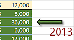
- In the section Block Arrows click on the Left Arrow.
The mouse pointer changes to the Precision shape. - Drag inside the cell you selected to create an arrow pointing
to the maximum value on the left. Make the arrow fit entirely within the cell borders.
 The
default shape has blue fill and darker blue outline.
The
default shape has blue fill and darker blue outline. - Save.
[trips24-Lastname-Firstname.xlsx]
AutoShape: Format
You can format a lot about a shape after you create one.
-
 With the arrow still selected, on the Drawing Tools: Format tab, click the Shape Fill button and choose Accent 6, Darker 25%.
 - Click the Shape Outline button and
choose Black as the color of the outline.
- Click the Shape Outline button again and choose Line Weight = 1 pt.
- Click the Shape Effects button and choose Shadow > Offset Diagonal
Bottom Right (the first choice in the Outer section).
- Click the Shape Effects button and choose Bevel > Circle (the
first choice after None).
- Save.
[trips24-Lastname-Firstname.xlsx]
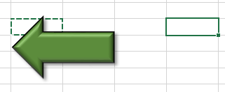
AutoShape: Copy with Cell
The AutoShape, like other drawings or images, is not actually in the cell. But, it is attached to the cell, as the following steps show.
-
 Select the cell (not the arrow itself
which will show resizing handles) containing the arrow and copy it.
Select the cell (not the arrow itself
which will show resizing handles) containing the arrow and copy it. - Select the Totals in the lower table, cells that are in column D.
- Inspect the Status Bar to see what the Max is for the selection.
- Select the cell in column F on the row to the right of the maximum
-
 Paste.
The arrow is pasted along with the cell.Of course you could have just selected the arrow itself and paste just the arrow. But doing it this way proves that the arrow was indeed attached to the cell since it came along for the ride when you copied the cell.
- Save.
[trips24-Lastname-Firstname.xlsx]
AutoShape: Delete
- While the cell is still selected
 , press DELETE to remove the arrow.
Nothing seems to happen. The arrow does not vanish! Only the cell contents would be deleted. The AutoShape is attached to the cell, but it is not counted as part of the cell's contents. -
Click on the arrow itself to select it.
The shape shows its resize and rotation handles.
- Press DELETE again. Now it is removed.
- Undo so that you again have two arrows on the sheet.
- Save.
[trips24-Lastname-Firstname.xlsx]
AutoShape: Copy with Cell?
What if the shape is larger than a single cell? If you copy one cell underneath the shape, will the shape be copied, too? It depends! When a shape or image is larger than two cells, you may need to select most of the cells underneath for copying to include the shape or image. Of course you could always copy and paste the shape or image separately if the first attempt fails.
Cutting cells works the same as far as whether or not an image or AutoShape will be included in the action.
- Experiment: Copying cells under a large AutoShape
 Copy and paste one of the arrow shapes to a blank area of the sheet.
- Drag a corner of the shape to enlarge it to cover at least two columns and 4 rows.
- Select the upper left cell underneath the arrow.
(Select a cell above the shape in the correct column and use the arrow keys to move the selection to the correct cell.)
 Copy and paste to a blank area.
The selected cell still has its dashed border. The arrow was not pasted along with the cell.- Repeat with different selections of cells under the arrow.
How many cells does it take for the arrow to be pasted?
Selecting over half the cells under the arrow seems to work most of the time - but not always!
|
|
| © 1997-2017 Jan Smith All Rights Reserved |
Site Map What's New |
Privacy Policy Terms of Service Copyright Acknowledgements |
~~ 1 Cor. 10:31 ...whatever you do, do it all for the glory of God. ~~
Last updated: March 22, 2017