Jan's Working with Numbers

Step-by-Step: Merges & Formulas

---

What you will learn:

to merge cells to repair formulas with absolute reference to repair formulas with AutoFill to repair formulas on sheets with linked cells

---

Start with: trips26-Lastname-Firstname.xlsx (saved in previous lesson)

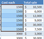
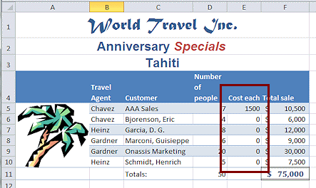
The Tahiti trip cost is $1500. It seems silly to enter that on the Specials sheet for each Tahiti trip. You will merge the cells for Cost each. BUT... this will break the formulas that calculate the Total Sale. So you will have to repair those formulas afterwards.

Format Cells: Merge

1. Open trips26-Lastname-Firstname.xlsx to the Agent Totals sheet.
   
2. Save As trips27-Lastname-Firstname.xlsx in the excel project4 folder of your Class disk.
3. On sheet Specials, select cells E5:E10, which all contain 1500, the cost of the Tahiti trip.
   
4. On the Home tab in the Alignment tab group, set Vertical alignment to Middle, and then click the button to Merge & Center.
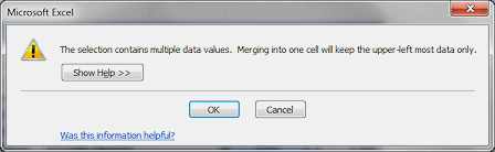
   Again you get the warning about losing data when you merge cells.
   

   

5. Click on OK in the message.
   

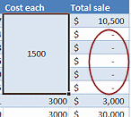
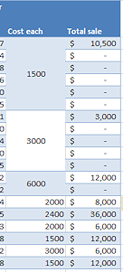
   Wipe out! A lot of cells lose their values.

   Effect 1: The formulas for Total sale use 'Cost each' from the cells that are now merged. Excel thinks that the merged cells are empty, except for the first one. You will fix this shortly.

   Effect 2: The Total at the bottom of the column is wrong, but the formula is not broken. It is adding up the column which now has a lot of zeros because you merged cells.
   

6. Repeat the procedure to merge the 'Cost each' cells for the New Zealand and World trips.
   (You can not do this for the group of Other trips because those trips do not all have the same value for Cost each.)

   It's looking good except for the background colors of the merged cells. They are not alternating like the rest of the table. The merged cells take the formatting of the upper left cell before the merge.
   

7. Click on the merged cell containing 6000 and copy.
   
8. Paste the formatting only to the merged cell containing 3000.
   The formatting apparently included merging just 2 cells. Unexpected!
   
9. Undo.

10. Click in the cell containing 3000 and from the Home ribbon tab, change the Fill Color to White.

    That one was easy because it is clear that the background was white. But in other situations Paste Formatting is better because you don't have to know what the colors are.

11. Click on the merged cell containing 1500 and copy.
    
12. Paste the formatting only to the merged cell containing 6000.
    This one worked as expected.
    
13. Press the ESC key to turn off the blinking selection.
    
14. Save.
    [trips27-Lastname-Firstname.xlsx]
    Your Cost each cells are neatly merged with alternating color for background. Next you will fix the broken formulas. 

---

Formula: Repair with Absolute Reference

The broken formulas for Total Sale use cells that vanished in the merge. You need to make the formulas refer to the remaining merged cell instead.

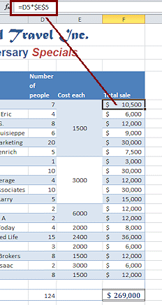
1. Select cell F5, which has a formula that still works.  =D5*E5 

   You need to change E5 in the formula to $E$5, an absolute reference, so you can use AutoFill for the other Total Sale formulas. You could edit it directly, but there is a shortcut.
   

2. In the Formula bar click next to E5 and press the function key F4, which for most keyboards is on the top row (above the number keys).
   E5 is changed to $E$5 so that the formula reads  =D5*$E$5 
3. Click the check mark to enter the new formula and keep the selection in F5.

   The F4 key will cycle the cell reference next to the cursor through the 4 possibilities:

   • relative cell reference E5
   • absolute cell reference $E$5
   • mixed reference with column absolute $E5
   • mixed reference with row absolute E$5
4. Save.
   [trips27-Lastname-Firstname.xlsx]  

---

Formula: Repair with AutoFill

Now that F5 has a formula that uses an absolute reference, you can use AutoFill to copy it into the other Total Sale cells for Tahiti trips.

1. With cell F5 selected, drag by the fill handle with the left mouse button to cell F10.

   AutoFill enters new formulas. These calculated values for Total sale are the same as before.
   But the background color from the first cell is copied down the column also.
   

2. Open the menu for the AutoFill Options button at the bottom right of the AutoFill selection.
   
3. Click on Fill Without Formatting.
   Success! Now the formulas work and the formatting is back to the original for
   column F.
4. Repeat the procedure for the New Zealand trips and the World trips.

   [Hint: Select the cell in Column F with a working formula. Edit it to use an absolute reference for the cell in column E. Drag by the fill handle to replace the other formulas for this agent. Fill without formatting.]
   

5. Center range E18:E23 to match the top of the column.
6. Save.
   [trips27-Lastname-Firstname.xlsx]  
7. In Print Preview, inspect your values and totals and fix any errors.
   Is the total still $269,000? If not, some of your test values were left behind when you were checking the linking.
8. Print the sheet Specials only.
   

---

Formula: Repair Linked Cells

Your changes on the sheet Specials also affected those sheets with cells linked to the cells you changed. You need to do some repair work on several sheets. Did you think about this effect?

1. Select the Tahiti sheet.

   Except for the first one, the Cost each cells show a zero since they are linked to merged cells. Data was lost in the merge. Whoops.

   The easy solution is to merge these cells, too.

   The Total sale values are still correct because those cells are linked to the cells you just fixed on the sheet Specials. They are not using cells on the Tahiti sheet at all! The joy of linking!
   

2. Select cells E5:E10  and set Vertical alignment to Middle, and then Merge & Center.
3. Repeat this procedure on the New Zealand and World sheets.
4. Similarly, merge the Cost each cells on Formatted Groups.
5. Center range E18:E23 on the sheet Formatted Groups.
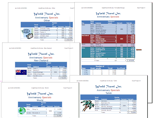6. Group the five sheets - Formatted Groups, Tahiti, New Zealand, World, Other.
7. Open Page Setup and on the Margins tab select Center Horizontally.

8. Check Print Preview for the correct centering, orientation, header, borders, etc. Make corrections if needed.

   If a sheet does not fit on one page, change the page break in Page Break Preview. Formatted Groups is probably putting the arrow in column G on a sheet by itself!
   

9. Save.
   [trips27-Lastname-Firstname.xlsx]  
10. Print active sheets to print the five active sheets.
11. After printing is finished, ungroup the sheets and close.