Jan's Working with Numbers

Step-by-Step: Copies & Formula

---

What you will learn:

to find out if a cell is a copy or if it is linked to change a copy to a link for labels and data cells to deal with merged cells when editing

---

Start with: trips25-Lastname-Firstname.xlsx (saved in previous lesson)

Copied or Linked?

When you are not sure if data is a copy or is linked, you have two methods for checking to see if the data is linked.

• Formula Bar: Click the cell and look in the Formula Bar to see if there is a formula there that shows the link to another sheet, like =Budget!A1.
• Test with changes: Actually make some changes in the original data and see if those changes show up on the other sheet.

It is probably faster and safer to look at the Formula bar, but only if you read the formula carefully to see which sheet is involved. This time you will make changes to the data and check to see that the change shows up elsewhere.

1. Open trips25-Lastname-Firstname.xlsx.
2. Save As trips26-Lastname-Firstname.xlsx in the excel project4 folder of your Class disk.
3. On the sheet Specials, change the number of people that AAA Sales bought trips for in cell D5 to 10.
4. Click the check mark on the Formula Bar to enter the new value so your selection will not move.
5. Select the sheet Agents Totals and expand the data by clicking the Level 3 button .
   Look at the value showing for AAA Sales. It is still 7.
   The sheet was not updated because it was a simple copy of the values.
6. Select sheet Tahiti and look in cell D5 at the number of people that AAA Sales bought trips for.
   This cell has been updated with the new number you entered. The data cells on this sheet are linked to the original data.
7. Undo your typing in D5.
   (You don't have to switch sheets to Undo. There is only one list of actions.) You should be moved back to the sheet Specials with 7 back in cell D5.
8. Select sheet Specials and change the value of cell E29 to 12.
9. Click the check mark to enter the new value.
10. Select sheet Tickets Sold Chart and look at the first bar.
    It has been updated with the new value, 12, for the sales in the first week. Chart values are linked to the original data.
11. Undo your change.
12. Experiment: Testing Links
    Make one change to the data on the sheet Specials. Look for changes on sheets that include that data or to the chart.
    Do you understand and remember what was linked to what?

    You don't have to remember and you don't have to change values to test! Look at the Formula bar. When you select a cell that is linked, the Formula bar will show a cell reference, like =Specials!C10. Don't forget to undo each of your changes to the data.

     If you are not sure you got all the changes reversed, close the file without saving it and then reopen it. You will be back to the last saved version. (You did save at the end of the last lesson, right?)

---

Change Copies to Links: Formatted Groups

The sheet Formatted Groups is a copy. What would it take to link these cells to the Specials sheet? There are a couple of issues to deal with but fixing the sheet Formatted Groups is not so bad.

You will have to handle the merged cells in column A separately.

Column labels

You will link the first column label and then use AutoFill to link the others.

1. On the sheet Formatted Groups, select cell A4, which contains the word 'Trip'.
2. Link this cell to A4 on the sheet Specials.
   [Hint: type  =  , switch to sheet Specials, click in cell A4 and press ENTER or click the check mark button.]
   You are switched back to Formatted Groups.
3. Drag the AutoFill handle for cell A4 on Formatted Groups to the right to F4.
   The row loses its height and the text no longer wraps.
4. While the labels are still selected, click the Wrap Text button .
   The row resizes to let the labels wrap.
5. Click in each cell in the row in turn.
   What does the Formula bar show? You should have cell reference formula, like =Specials!F4
   
6. Save.
   [trips26-Lastname-Firstname.xlsx]
   

Data cells

1. On the sheet Specials, select range A4:F4 and AutoFill the whole table.
   [Hint: Drag the selection down to row 25.]
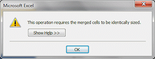
   A message appears. You can't do this because of the merged cells. Rats!
    
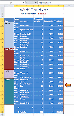2. Select instead range B4:F4.
   There are no merged cells in this range.
3. AutoFill by dragging the AutoFill handle of the selection to row 25.

   Is this a 'Whoops'? You did not want the formatting copied!
   If you act NOW, it's not a problem but just a step along the way.
   

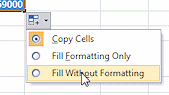4. Hover over the AutoFill Options button at the bottom right of the range and click the arrow to open the menu.
   The menu of options appears.
   
5. Click on Fill Without Formatting.
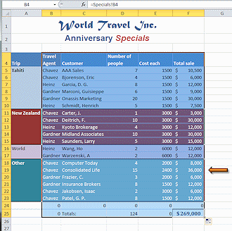   All the label formatting vanishes and the values are the same except some new zeros. 

   Better! The only problem is the zeros that appear in some blank spaces.

6. Remove the zeros from rows 24 and 25 since they are not necessary.
   
7. Save.
   [trips26-Lastname-Firstname.xlsx]
    

Merged cells

1. On the sheet Formatted Groups, select cell A5, which contains the word Tahiti.
2. To link this cell, type  =  , switch to sheet Specials, click in cell A5, and click the check mark on the Formula Bar.
   You are switched back to the sheet Formatted Groups, still in cell A5. Look at the Formula Bar.
   The cells are linked.
3. Repeat to link cells A11, A16, and A18 on Formatted Groups to the matching cells on sheet Specials.
4. Use the key combo CTRL + ` to show formulas.
   All the cells in the top table that show a cell reference formula are linked. Only the title cells in rows 1 and 2 should be unlinked.

   If you link the title cells, you will lose the separate formatting for the word Specials. We'll leave well enough alone in this case!

5. Hide the formulas by using the key combo again, CTRL + `
   
6. Save.
   [trips26-Lastname-Firstname.xlsx