Jan's Working with Numbers

Step-by-Step: Select Cell

---

What you will learn:

to select a cell with the mouse                          with keys                          by cell reference                          by name to create a cell name to select all cells to select all data cells

---

Start with: budget-2010-Lastname-Firstname.xlsx from the previous lesson

---

You will not be saving the file during this lesson. You are just selecting various cells. Later lessons require these methods so you do not need to save or do screen captures during this one.

Excel 2013 and 2016 have different colors for highlighting what is selected.

Select Cell: Mouse

Clicking any cell selects it. Sometimes the problem is to get to the cell.

1. If necessary, open the spreadsheet you saved in the last lesson, budget-2010-Lastname-Firstname.xlsx
   Be sure that the tab Budget at the bottom of the window is selected. It should be white.
   

2. Click on cell C4 to select it.
   (It's the intersection of column C and row 4.)

   

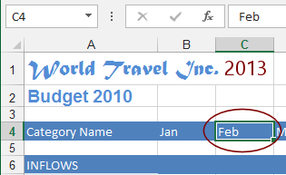
   Changes on selecting:

   • Cell border is in a contrasting color.
   • Name Box shows the cell reference, C4.
   • Formula bar shows the cell's contents, text = Feb.
   • The row and column headings for the cell change color.

   Now that you have seen how Excel 2013 and 2016 use different colors, we will show only one set of illustrations in most situations.

3. Scroll down until cell A44 is at the top of the sheet window.

   The scroll box will only scroll the screen to the last row with data in it is showing. To scroll blank cells into view, use the scroll arrow or the scroll wheel on your mouse.
   

4. Click cell A45 to select it.

   It can take a bit of work to get to some cells!

---

Select Cell:  Keys 

Let's practice moving around a spreadsheet using keys. Check the row heading and column headings and the Name Box as you follow the directions below to be sure you are in the correct cell.

1. Press TAB repeatedly to move once column at a time to the right, until cell E45 shows the dark border for a selected cell. 
   Notice that the row and column headings of the selected cell are colored.
2. Press the UP arrow key repeatedly to move the selection to E20.
3. Press the RIGHT arrow key repeatedly to move the selection to J20.
4. Press the HOME key to move the selection to A20, the beginning of the row.
5. Use the key combo CTRL + HOME to move the top left of the sheet - cell A1.
6. Press END and then right arrow to move to the end of the row -cell XFD1.
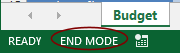   Did you notice that the Status Bar shows End mode at the bottom left? Keys behave a bit differently in End Mode.
7. Press CTRL + END to move to the last cell with data, at the bottom right, N46.
8. Press END and then the down arrow to move to the end of the column - cell N1048576.
9. Press END and then left arrow to move to the beginning of the row again - cell A1048576.
   
10. Press  CTRL + HOME to return to cell A1.
    
11. Press END and then the down arrow.
    The selection moves down just one row to A2.
    
12. Click on the cell Inflows (A6). Press END and the down arrow again.
    The selection jumps! In END mode, the selection will move to the end of the 'section'.
    
13. Experiment: Key Combos for navigation
    Practice moving around the spreadsheet with the different key combos you just learned.
    Can you discover others?

---

Select Cell: Cell Reference

By using the Name Box you can avoid long scrolls.

1. Click in the Name Box on the Formula Bar and type the cell reference N46 

   You don't have to use capital letters in cell references.
   

2. Press ENTER.
   You are moved directly to that cell. (This is cool!)

   
   

3. Scroll up using the scroll box until you see Row 10.
   (Watch the  screen tip while you are scrolling.)
     
4. Scroll to the left using the horizontal scroll bar until you see Column A.
   The selected cell is still N46, as shown by what is in the Name Box.
   Scrolling does NOT change the selection.
5. Use the key combo CTRL + BACKSPACE to return to the selected cell, still N46.
6. Press CTRL + HOME to move back to the top of the sheet and select cell A1.
   

---

Select Cell: Create and Use a Name

Name special cells and ranges that you move to often. Names are so much easier to remember than columns and rows, which can change if you add or remove data!

Name a cell

1. Select cell N44.
2. Click in the Name Box and type Total Inflow 2010
   
3. Press ENTER.
   Whoops. You will see an error message. The problem is the spaces in the name.
4. Click on OK in the message window.
5. Retype the name as TotalInflow2010 and press ENTER.
   This works fine.
6. Return the selection to cell A1.
7. Drop the list for the Name Box by clicking its arrow.

Problem: Named a cell incorrectly
You cannot remove a name from the drop list here but there is a way.
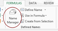
Solution: On the Formulas ribbon tab in the Defined Names tab group, click on Name Manager. Select the name that is wrong and click on Delete.

Navigate by cell name 

1. Click on  TotalInflow2010.
   You are immediately moved the cell with that name - N44.
   
2. Experiment: Using named cell/region
   • Drop the list of named cells again and select a different one.
   • If necessary, scroll or use CTRL + BACKSPACE to see exactly what was selected.
     

   • Repeat to check out each choice.

     A name can refer to a single cell, like TotalGrossSales or to a range, like AugustInflows and Print_Area.
     

   • Pick a cell and name it. Then move away from it. Move back to it, using the name.
     

---

Select Cells: Select All

There is a quick way to select all the cells on the sheet. This is useful when you need to copy everything to another sheet or another workbook. But you have to know where to look!

1. Click on the Select All button, which is the intersection of the column and row headings.
   The button has a small arrow head that points down and right.

   All cells on the sheet are selected, not just the ones you have worked with and not just the ones you see in the window.

   Warning: Odd Name Box behavior
   The Name Box shows the cell reference or the name of the top left cell that is showing after you use the Select All button, NOT the top left cell of the range that is actually selected! Your window may show a different cell at the top left than the illustration, depending on your window's size.

   Selecting the whole sheet can be dangerous. It might seem logical to format the whole sheet at once. Don't! Formatting 1,048,576 rows in 16,384 columns can take a very, VERY long time to complete. Format only what you really need to format. Formatted cells may try to print, even when they are empty!
   

2. Click in a cell to remove the selection.

---

Select Cells: Select All Data Cells

Sometimes you need to select all of the cells that actually contain something and not the blank cells in the rest of the worksheet. There is a key combo for that.

1. Use the key combo CTRL + HOME to return to cell A1.
   
2. Use the key combo SHIFT + CTRL + END to select from the selected cell to the last cell that actually has data.
   All cells from A1 to the last used cell are selected.
   
3. Click in a cell or press the ESC key to remove the selection.