Format & Arrange:
Exercise Excel 3-2

Start with: , soccer budget2.xls (created in previous exercise)

You will practice moving, inserting, and formatting by making changes to soccer budget.xls, which you previously created in Exercise 2-2. You will include new columns for the calculations that were used to get certain budget amounts.

1. From your Class disk open  soccer budget.xls  in the excel project2 folder to Sheet1.
    
2. Save to your Class disk in the excel project3 folder with the name  soccer budget3.xls 
    
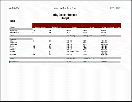
3. Move: Move the Income cells, including the Totals, to be above the Expenses cells. [Hint: Cut and Insert Cells.] There should be a blank row between the Totals and Expenses rows. Move the column labels from below Expenses to above Income.
    
4. Insert: Between the columns Category and Budget, insert 2 columns. Label the columns Budget Quantity and Budget Cost each and wrap the text. These will be used to calculate the Budget column.
   
   Below the Trophies row insert a blank row for a second type of trophy.
    
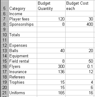5. Enter Data: Use the numbers in the illustration on the right to fill in the data in the new columns.
    
6. Repair Budget formulas: In the Budget column, replace the values, wherever values exist in both Budget Quantity and Budget Cost each, with a formula. [Multiply the Budget Quantity by the Budget Cost each.] For Trophies, add together the cost of the two types of trophies for the Budget column.
    
7. Format: Cells A1, A2,and A3 use the font Impact and are merged and centered across the table. Font size for A1 = 22, A2 and A3 = 18. Make all of the row labels in Column A Bold.
    
8. Cell Style: Create a cell style for the column labels named Label - white on red: Fill = Dark Red, Font Color = White, Font = Arial, Font Size = 10, Centered, Bold, Wrap Text. Apply this style to the column labels in row 5. Widen the columns as necessary.
    
9. Cell Style: Create another cell style for the Totals rows named Totals. (Select cell D10 to base the style on and the current number format will be retained.) Use Font = Arial, Font Size = 10, Bold, Font Color = Blue, Fill Color = Gray 25%. Apply the style to the table cells in the Totals rows and also to the cells containing the words Income and Expenses.
    
10. Revise Over/Under Formulas: The last column is supposed to show how the actual income and expenses compare to the budgeted amounts. Being "over budget" for expenses is a bad thing. But being "over budget" for income is good since you earned more money than expected. This is confusing! You need a different approach.
    
    Change the column label to read Difference = Actual - Budget.
    Change all the formulas in column F to =Actual - Budget (Yes, you can really use column labels in your formulas!) If you lose styles, reapply the style.
     
    Error?: If you see #NAME? in the cell instead of a number, your Excel is not set to allow using labels in formulas. Change this by choosing Tools | Options and, on the Calculations tab, check the box for "Accept labels in formulas".
     
11. Grand Totals: Leave  a blank row below the expense Totals row and create a Grand Totals row below it. Type Grand Totals: in column A of the new row. In cells columns E and D write formulas that subtract the Expenses value from the Income value in that column. In column F use the same formula as in the rest of Column F, =Actual - Budget. Format the Grand Totals row with the Totals style and border it with a dark wide border.
     
12. Rename Sheet: Change the name of Sheet1 to Soccer Budget and of Sheet2 to Budget Charts.
     
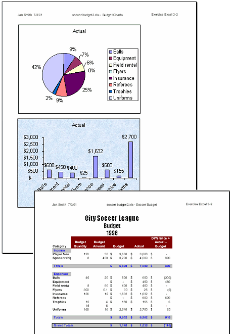
13. Charts: On the sheet Budget Charts, there is an extra square in the Legend because you added a row for the second type of trophy. Change the Source Data, reselecting the labels cells and the values cells and omitting the blanks that are causing the problem. [Hint: Hold CTRL down while you select the cells.] Copy the existing pie chart and paste it below on the same sheet. Change the Chart Type of the copy to Column. Do not show the legend. Format the chart area with the Fill Effect texture Blue tissue paper. [Format Chart Area | Pattern | Fill Effects | Texture. If the texture named is not available, choose another one.] If necessary, change the font size for the axis labels and resize the chart area to make the chart easy to read.
     
14. Prepare to print: Edit the header for both sheets to show Exercise Excel 3-2. Spell Check. Page Break Preview. Print Preview. (Each sheet should fit on one page) Fix any problems.
     
15. Save. [soccer budget3.xls]
     
16. Print the Entire workbook.
     
17. Print formulas: Show formulas and print the Soccer Budget sheet only, in Landscape orientation on a single page.
     
18. When all printing is complete, close the workbook without saving again.