Format & Arrange:
Exercise Excel 3-3

Start with: , amazon pings2.xls (created in previous exercise)

The spreadsheet amazon pings2.xls [created in Exercise Excel 2-3] contains the records of a series of tests (over several weeks) of Internet speed to the Amazon.com site. Each test measures the time for a signal to make the round trip to amazon.com and back. This signal is called a "ping".

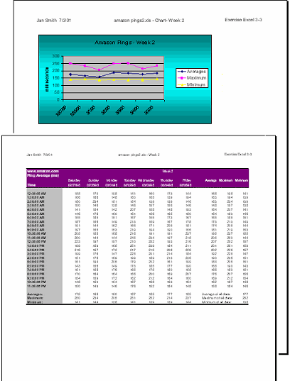
You will create a sheet for the data for a single week, along with a chart of average, maximum, and minimum ping times for each day.

1. From your Class disk open the file amazon pings2.xls that you saved in the excel project2 folder for Exercise Excel 2-3.
    
2. Save As with the name  amazon pings3.xls  to the folder excel project3.
    
3. Paste Link: In Normal view, copy the titles and labels in Column A and Paste Special… | Paste Link them to Sheet2 in cell A1. Copy the data for the second week - J1:P33 - and Paste Link to cell C1.
    
4. Edit: Delete all the zeros that appear where there were blank cells originally.
    
5. Format: Using Format Cells… | Number,
      Time- Format cells A6:A29 as time like 1:30:55 PM.
      Date- Format cells C4:I4 as dates like 03/04/97.
      Data- Format the data cells and calculated values as Number with 0 decimals.
    
6. Enter data: In cell G1 type Week 2. In cell K3 type Average, in L3 type Maximum, in M3 type Minimum. In cell K31 type Average of all data:, in cell K32 type Maximum of all data:, in cell K33 type Minimum of all data:
    
7. Formulas: Create formulas - in cell K6 to average the data in that row, in cell L6 to find the maximum value in the row, and in cell M6 to find the minimum value in the row. Copy these formulas down the column for each hour of the day.
    
   Write a formula in cell M31 for the average of all of the data cells, in cell M32 to find the maximum, and in cell M33 for the minimum.
    
8. AutoFormat: Apply the table format Classic 2 to the entire table (but not the whole page!)
    
9. Resize: Resize columns K, L, and M to 8.00 but be sure that the labels in K31:K33 show completely. Resize Columns J to 2.00 to help reduce the table's width.
    
10. Chart: Select the dates across the top and the values at the bottom of those columns for Averages, Maximum, and Minimum. Use the Chart Wizard to create a Line chart with markers at each data point. On the Series tab, name Series 1 = Average, Series 2 = Maximum, Series 3 = Minimum. Set the title = Amazon Pings - Week 2 and the Value (Y) Axis = milliseconds. Place the chart as an object in Sheet 3. Drag the chart to the upper left of Sheet3.
     
11. Format Chart: Format the Chart area with Fill Effect | Gradient using Light Turquoise and Aqua as the two colors. Select the Horizontal gradient that is light in the middle and darker at the top and bottom.
     
12. Rename sheets: Change the name of Sheet1 to Original Data, Sheet2 to Week 2, Sheet3 to Chart.
     
13. Prepare to print: Create or edit the header for each sheet to include your name and date in the Left section, file and sheet name in the Center section, and Exercise Excel 3-3 in the Right section. Spell Check. View Page Break Preview and/or Print Preview for sheets Week 2 and Chart - Week 2. Select the sheet Week 2 and set Page Setup | Page to print To fit 1 page wide by 1 page tall. Select sheet Chart - Week 2 and set Page Setup | Page to print at scaling = 100%.
     
14. Save. [amazon pings3.xls]
     
15. Print: Group sheets Week 2 and Chart - Week 2 and print the two active sheets. Check the print preview to be sure your Page Setup choices are still there. You should have two pages only.