
Jan's Working with Numbers
Design: Analysis: Print Comments
 When you print your
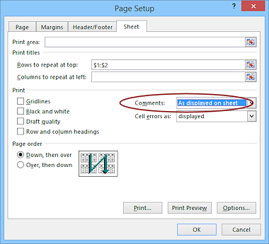
worksheet, do you want to see the comments or not? Printing choices
for comments are on Page Setup's Sheet tab.
When you print your
worksheet, do you want to see the comments or not? Printing choices
for comments are on Page Setup's Sheet tab.
Your choices for printing:
-
(None) = no comments printed, which is the default.
-
All comments printed at the end of sheet on a separate page
-
As displayed on the sheet (only the ones that are visible)
Comment Order
Comments are named in order, as you create them, with boring default names: Comment 1, Comment 2, etc. This is the name that shows in the Name Box when the comment is selected. You can rename a comment just like you can name a cell. Select the comment and type the name in the Name Box. The names won't print, so usually there is not much point in changing the default names.
If you choose to print comments "at end of sheet", they appear in cell order (by row, then column) rather than the order in which you created them and thus the way they are numbered. The comments attached to the three cells in the illustration were created in the order A1, C3, and C1 but are not printed that way.

Three comments; Printed at end of sheet in order by row, then column
![]() Best
location for comments: Cell A1 is normally where hidden comments about the sheet as a whole belong. Reserve comments in other cells for explanations of that cell's importance or its behavior or its data source. For visible comments choose a cell that will let the comment display nicely
without hiding your data.
Best
location for comments: Cell A1 is normally where hidden comments about the sheet as a whole belong. Reserve comments in other cells for explanations of that cell's importance or its behavior or its data source. For visible comments choose a cell that will let the comment display nicely
without hiding your data.
| |
Step-by-Step: Print Comments |
|
| What you will learn: | to make comments always visible to paste text into a comment to adjust an AutoShape with adjustment handles to zoom the view and see temporary formatting changes to move a comment to print comments as displayed to print comments together at the end to hide comments |
Start with: ![]() trips31-Lastname-Firstname.xlsx - sheet Specials (saved
in previous lesson)
trips31-Lastname-Firstname.xlsx - sheet Specials (saved
in previous lesson)
Comment: Visible
-
 Open Excel Options.
 Office button or File tab > Excel Options or Options
-
On the Advanced page in the Display section, click the radio button to show Comments and indicators.
Now your comments will be visible all the time.When comments are showing all the time, you must be careful about where you position comments. You don't want them to hide the sheet data.
-
Click on OK to close the dialog and apply your change.
This option setting applies to ALL Excel spreadsheets, not just this one, and shows ALL comments.
Alternate method: Show a particular comment ALL the time
Right click the cell to which the comment is attached and choose Show Comment.
Comment: Paste Text
You can put your Analysis in a comment instead of in cells. You don't even have to type it over again! You can copy and paste it to your comment.
- Open trips31-Lastname-Firstname.xlsx, if necessary.
-
 Save As trips32-Lastname-Firstname.xlsx to your Class disk in the
folder excel project5.
Save As trips32-Lastname-Firstname.xlsx to your Class disk in the
folder excel project5.
- Double-click cell A50 to edit it.
-
Drag to select all of the text in cell A50 (your analysis) and then Copy.
If you try to copy the cell instead of the cell contents, nothing will happen when you paste to the comment box.
The key combo CTRL + A does not work to select all of the cell's contents.
- Click in a cell to unselect A50.
-
Click on the comment attached to cell G1.
Your comment should be visible all the time now. - Delete the line in the comment starting 'Purpose: to show..."
That information is already in your Analysis. - If necessary, put the cursor at the end of the comment text and press ENTER to create a new line.
- Paste.
The text from cell A50 appears at the end of the comment.
- Format your pasted text by making Analysis: bold.
Add other formatting and blank lines, if you wish, to make your text easier to read. -
Resize the comment's text box in width and length to show all the text.
Your comment box may need to be a different size from the illustration, depending on how long your analysis is.
 Zoom
changes wrapping - but not really: Look at cell B4 and D4 in
the illustration. The text is wrapping oddly.
This screenshot was taken with the sheets shown at less than 100% zoom.
Apparently Excel will change font size and text wrapping as the display
gets smaller and smaller to keep the labels readable as long as
possible.
Zoom
changes wrapping - but not really: Look at cell B4 and D4 in
the illustration. The text is wrapping oddly.
This screenshot was taken with the sheets shown at less than 100% zoom.
Apparently Excel will change font size and text wrapping as the display
gets smaller and smaller to keep the labels readable as long as
possible. -
 Experiment: Zoom
Slide the Zoom control at the bottom right of the Excel window and watch how Excel manages the display at different zoom levels.
Data cells may cut off characters or show #### hash marks for numbers. Labels will be cut off or wrap oddly. The title will change to a simple font.
 Excel 2010: At some small
zoom number 'Table 1' suddenly appears across your table.
Excel 2010: At some small
zoom number 'Table 1' suddenly appears across your table.The illustration shows 28% zoom, but your screen may look quite different at 28%. It depends on the size of your monitor's screen and the resolution your monitor is running.
Check
Print Preview at 100% before panicking.
Zooming can distort what you see. Those ### hash marks can show up in a zoomed view even though the cells will print just fine. Borders often do not show in a zoomed view correctly. Text can even wrap incorrectly.When you are ready to continue, return to 100% zoom.
- Select A50 again and delete its contents and then AutoFit row 50 and unmerge the merged cells.
- Save.
[trips32-Lastname-Firstname.xlsx]
Adjust Shape
 The shape for this comment has 3 yellow adjustment handles. You may not be able to see the one at the top since this shape bumps up against the top of the spreadsheet.
A shape may have no adjustment handles at all or just 1 or 2.
The shape for this comment has 3 yellow adjustment handles. You may not be able to see the one at the top since this shape bumps up against the top of the spreadsheet.
A shape may have no adjustment handles at all or just 1 or 2.
The handle on the top edge of the shape controls the length of the arrow. A handle on the arrow itself controls the thickness of the shaft of the arrow. On the left edge of the shape, a handle controls the size of the arrow head. You will change the size of the arrow to make it less bulky.
Your shape may have different height and width than what the illustration shows.
-
 Drag the shape down to
so that it's top edge is in row 2.
Drag the shape down to
so that it's top edge is in row 2.
Now you can see the adjustment handle at the top and the rotation handle.
- Experiment: Adjust Shape
Drag each of the yellow adjustment handles around to see what they can do.
How weird a shape can you create?
When you are ready to continue...
- Drag the handle of the top edge to make the
text start at the right edge of column H.
- Drag an adjustment handle on the arrow's shaft to make the shaft about two
normal rows tall and half the width of column H.
- Drag the adjustment handle on the left edge of
the comment to make the arrow's head about
4 rows at its widest point.
- Drag the shape back up to the top of the sheet.
Comment: Move Comment
A comment will normally move when you move the cell to which it is attached. But what if you want to move the comment but not the cell contents? It takes an extra step or two.
You will move your comment in cell G1 to cell A1 without overwriting that cell's contents. It's a three step process - copy, paste special to new cell, delete old comment.
Unexpectedly, you cannot select a comment and cut or copy and
then paste. The Cut and Copy commands are grayed out when a comment is
selected!
 Select cell G1. Copy.
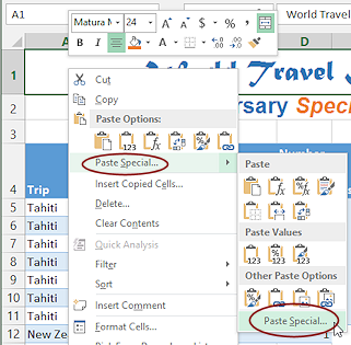
- Right click on cell A1.
- On context menu, hover over Paste Special to expand the palette of paste icons.
There is no icon for the Paste Special dialog. - Click on on the command Paste Special...
The Paste Special dialog opens.
-
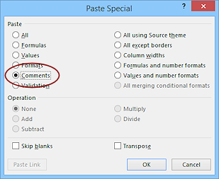 Click on Comments and then on OK.
Your comment is pasted, but only the comment - not the cell's contents or formatting. Since Excel is currently set to always show comments, you can see both copies. Weird looking, isn't it? Both A1 and G1 show the
red triangle in the upper right corner.
Both A1 and G1 show the
red triangle in the upper right corner.
- Click on G1 and press the DELETE key.
Nothing happens. G1 was already blank and the comment is still there. Deleting a cell's contents does not delete an attached comment.
-
 Right click on G1
and from the context menu select Delete Comment.
Right click on G1
and from the context menu select Delete Comment.
Alternate Method to Delete Comment: Select the comment (In Excel 2007 and 2010 it will have a dotted border) and press the DELETE key. But in this situation, with the two comments overlapping it is very easy to select and delete the wrong one.
- Save.
[trips32-Lastname-Firstname.xlsx]
Comment: Print as Displayed
You control how comments print from the Page Setup dialog on the Sheet tab.
 Open Page Setup.
- On the Sheet tab, for Comments select As displayed on sheet.
- If necessary, set Rows to repeat at the top to $1:$2 to get the
title cells on all the pages.
- If necessary, on the Page tab select Portrait orientation and
set Scaling to 100%.
- Click OK to close the dialog and apply your
changes.
-
 Open
the Page Break Preview.
Open
the Page Break Preview.
If necessary, insert a page break between the two tables.If necessary, drag the right border wide enough to include the whole comment.
Make sure that only 2 pages will print and all of the data and the comment will print.
- Open Print Preview and check all pages.
This is not quite what you want! Page 1 is OK, though perhaps a bit small. But page 2 looks very odd. Part of the comment is showing because you are repeating rows 1 and 2 on each sheet and the comment overlaps those rows. <sigh>
-
Close Print Preview and return to Normal view.
- Drag the comment box down so that it does not overlap the repeated rows
1 and 2.
- Check Print Preview again.
Looks much better!
 Print the
page 1 only.
Print the
page 1 only.
- Save.
[trips32-Lastname-Firstname.xlsx]
Comment: Print at End
Printing comments at the end has the advantage of putting all your comments together. It may also simplify your formatting since the comments, whether hidden or visible, will not print on the pages with data.
-
 Open Page Setup again to the Sheet tab.
- For Comments select At the end of sheet
- Open Print Preview.
The comment is on page 3. Any formatting you applied to the comment box does not show up in print! This is VERY plain text.
- Print page 3 only to print just the
page with the comment.
- Print.
Comment: Hide
- Open Excel Options again to the Advanced setting and under Display, click the radio button for showing No
comments or indicators.
- Click on OK to apply your settings.
Now the comment indicator is hidden and so is your comment.
- Right click on A1 and select Edit Comment.
The comment shows up. When a user looks at this sheet, there is no clue that there is a hidden comment. Sometimes that is a good thing and sometimes it's not. - Open Excel Options again and change the setting for Comments back
to Indicators only, and comments on hover.
These setting change the way Excel behaves all the time, so you don't want to leave an unusual choice in place once you no longer need it.
- Click on OK to save your change.
- Save.
[trips32-Lastname-Firstname.xlsx]
|
|
| © 1997-2017 Jan Smith All Rights Reserved |
Site Map What's New |
Privacy Policy Terms of Service Copyright Acknowledgements |
~~ 1 Cor. 10:31 ...whatever you do, do it all for the glory of God. ~~
Last updated: March 22, 2017