
Jan's Working with Numbers
Design: Analysis: Comments
One way to include your documentation without cluttering up the worksheet is to use comments.
Excel lets you insert a comment into any cell. The comment acts like a hidden sticky note.
By default, a cell that has a comment displays a small red triangle in the upper right of the cell.
Make a comment appear:
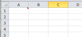
![]() Move your mouse
over cell A1 in the illustration.
Move your mouse
over cell A1 in the illustration.
The comment pops into view. When you move the mouse out of the cell, the comment vanishes again.
(If this did not work for you, your browser does not allow JavaScript from onMouseOver and onMouseOut commands.)
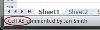 Most
comments are hidden until you select or hover over the cell. The Status bar
changes to show that the selected cell has a comment.
Most
comments are hidden until you select or hover over the cell. The Status bar
changes to show that the selected cell has a comment.
Working with Comments
The Default Comment
Excel 2007, 2010, 2013, and 2016 all have the same default comment, except for the shadow.
- Shape: Rectangle
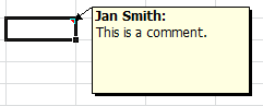
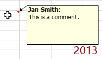
- Size: about 4 rows tall and 2.5 columns wide
(for default row and column sizes) - Background Color: pale yellow
- Border: thin, black
- Font: Tahoma, 9 pt, black
- Author: Bold, Tahoma, 9 pt, black
Automatically inserts the user name for Office, not the document's author - Shadow:

 narrow, down right;

 no shadow
 - Location: Pops up at the right of the cell with its top a little higher than the top of the cell.
![]() Author shown is not you: If your name
is not showing as the comment's author, you can delete the name and retype.
If you expect to do a number of comments (and you are working in your own
copy of Excel!), change the user name in Excel
Options > General. Then you won't have to retype
each time you create a comment. This change will be picked up by ALL Office programs, so be
careful.
Author shown is not you: If your name
is not showing as the comment's author, you can delete the name and retype.
If you expect to do a number of comments (and you are working in your own
copy of Excel!), change the user name in Excel
Options > General. Then you won't have to retype
each time you create a comment. This change will be picked up by ALL Office programs, so be
careful.
![]() Excel
remembers the position for editing: If you need to
see underneath a comment that is always open, you can
drag the comment by its border to a new position. The next time the comment pops up, it will be back in the default location - to the right of the cell with the comment's top edge slightly above the cell.
When you next edit the comment, however, it will move to where you left it the last time you edited. A bit confusing... but actually handy!
Excel
remembers the position for editing: If you need to
see underneath a comment that is always open, you can
drag the comment by its border to a new position. The next time the comment pops up, it will be back in the default location - to the right of the cell with the comment's top edge slightly above the cell.
When you next edit the comment, however, it will move to where you left it the last time you edited. A bit confusing... but actually handy!
| |
Step-by-Step: Comments |
|
| What you will learn: | to create a comment to format a comment - fill and font color to edit an existing comment to use keyboard shortcut in a comment to add a command not on the ribbon to the Quick Access Toolbar to change the shape of a comment |
Start with: ![]() trips30-Lastname-Firstname.xlsx - sheet Specials (saved
in previous lesson)
trips30-Lastname-Firstname.xlsx - sheet Specials (saved
in previous lesson)
Comment: Create
Comments about the sheet as a whole are usually put in cell A1. However, for some sheets, such a comment could not be visible all the time without blocking part of the sheet.
- Open trips30-Lastname-Firstname.xlsx if necessary, to the sheet Specials.
-
 Save As trips31-Lastname-Firstname.xlsx to your Class disk in the
folder excel project5.
Save As trips31-Lastname-Firstname.xlsx to your Class disk in the
folder excel project5. - Select cell G1.
-


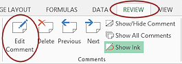
 From the ribbon tab Review in the Comments tab group, click the
button New Comment .
From the ribbon tab Review in the Comments tab group, click the
button New Comment .
The default comment box appears with handles for resizing and a cursor ready for your typing.The comment box is ready for typing when...
Excel 2007, 2010: Border of the comment shows diagonals and resizing handles.
Excel 2013, 2016: Border of the comment shows resizing handles. It will always have a plain border.
 If necessary, change the user name to your own
name.
If necessary, change the user name to your own
name.
-
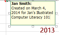
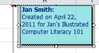
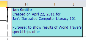
Below the user name, type Created on and type the date, a space, and then the word for , a space, and then the name of the class you are doing this sheet for.
You can't use Insert > Date like you can in the Header/Footer. If you are not sure of the date, hover over the time in the Windows tray at the bottom right of your screen. The date will popup if it is not already showing.
- Click in an empty cell to close the comment.
Next you will format your comment.
Comment: Format
The Review ribbon tab has a Comments tab group for managing your comments. You can also right click on a cell with a comment to get some of these commands.
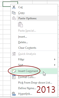 For comparison, right click on cell H1, which does not have a comment.
The context menu includes the command Insert Comment.
You don't need to create one at the moment.
-
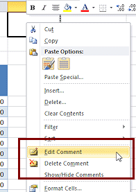 Right
click on cell G1.
Right
click on cell G1.
The context menu appears. Since this cell already has a comment attached, the choices are different than before.Notice that this menu also includes Edit Comment, Delete Comment and Show/Hide Comment.
Show means that the comment will stay open when you move on to other cells. Hide means to return the comment to its normal behavior - vanishing when the cell is no longer selected. This command is a toggle - click it once to Show and click again to Hide.
On the Review tab there is a button, which does not show on the context menu, that will show all comments on the sheet at once or hide them all.
- Select Edit Comment.
The comment pops into view with handles on the border and the cursor is blinking. You are in Edit mode for the text. -
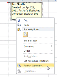 Format comment: Right click on the border of the open comment and from the context menu, select Format Comment.
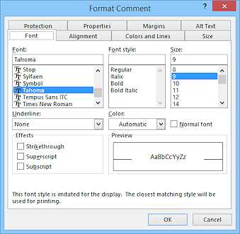 The Format Comment dialog appears, with several tabs.
 Problem:
Dialog has only one tab
Problem:
Dialog has only one tab
You missed the border with your right click and click inside the comment. You opened the dialog to format the text inside the comment.
Solution: Close the dialog and right click the border of the dialog.Problem:
Comment closed
You missed with your right click and clicked outside the comment.
Solution: Just repeat the steps above to open the comment up and try again. -
On the Colors and Lines tab, set the Fill Color to Aqua and the Fill Transparency to 50%.
Leave the line color as Black.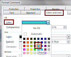
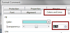
The transparency lightens the color and lets the grid lines or whatever is underneath show through. This can be helpful for comments that pop up over data cells.
Palette of colors: Did you notice the colors ono the color palette? These are not the Theme colors. This is the old color palette. This makes it more difficult to match the colors to other colors on the sheet.

-
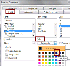 On the Font tab, set the Font Color to Dark Blue.
 - Click on OK to close the dialog and apply your
changes.
- Click on any cell to close the comment.
Comment: Edit Text
Next you will add some text to the existing comment.
- Click on cell G1.
-
On the Review tab click on the button Edit Comment.
The comment box appears with a cursor at the end of the existing text, ready for your editing.
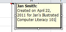
- Create a line break: Put the cursor to the left of your course's name and use the key
combo SHIFT + ENTER to create a line break.
This puts the course name on a line by itself.
-
 Create a new line: Put
the cursor at the end of the course name and press ENTER twice to create a blank line and a new 'paragraph', just
like in Word.
Create a new line: Put
the cursor at the end of the course name and press ENTER twice to create a blank line and a new 'paragraph', just
like in Word.
 Point of
Confusion: Different key combos for cells and for comments
Point of
Confusion: Different key combos for cells and for comments
In a cell you create a line break with ALT + ENTER. You cannot create a 'paragraph' in a cell. Pressing ENTER records the cell's contents and moves the selection to a new cell.
In a comment the usual Word keys work: SHIFT + ENTER for a line break and ENTER for a paragraph break.
- Type: Purpose: to show results of World Travel's special trips offer
- Resize the comment box to cover the range H1:J3.
The transparency of the background color for the comment helps here since you can see the grid lines underneath.
- Click on an empty cell to close the Comment box.
- Save.
[trips31-Lastname-Firstname.xlsx]
Add Command Not On The Ribbon to Quick Access Toolbar
You can change the plain rectangle shape for a comment but it's not as easy as in earlier versions of Excel. The Drawing Tools tab does not appear when you select the comment even though the comment is a text box shape.
You will add a command to the Quick Access Toolbar. In Excel 2010, 2013, and 2016 you have an additional option. You could add the command to a custom ribbon tab or to an existing tab (like the Review tab) in a custom tab group.
-
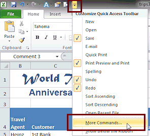 Click on the More button at the right end of the Quick
Access Toolbar.
Click on the More button at the right end of the Quick
Access Toolbar.
A menu appears. The first items are commands that many users want to see on the Quick Access Toolbar. A check mark means that item is already on the bar.This screenshot shows a bar with some additional items that are not on the quick pick list.
- Click on More Commands...
The Excel Options dialog opens to the Customize Quick Access Toolbar tab.
-
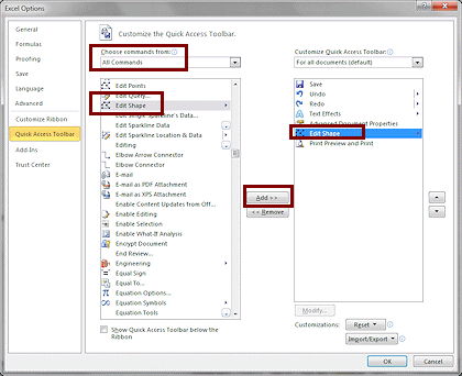 Change the box for Choose commands from: to All Commands.
The command you want is Edit Shape, which appears on the Drawing Tools: Format tab. But that ribbon tab does not show up for a Comment. Annoying! Since the command is not in the list of Commands not in the Ribbon, you have to pick All Commands or Commands Not on the Ribbon to find it.
- Scroll the list of commands to see how many different commands there are. When you are ready to continue...
- Click on
 Edit Shape.
The arrow at the right of the command means that the button will have an arrow to drop a list of choices. - Click on the Add>> button in the middle of the
dialog.
The command appears in the list on the right of items on the Quick Access Toolbar at the bottom of the list.
-
Click the Up arrow to the right of the list to move Edit Shape up one spot.
Alternate Method: First select the toolbar item in the list on the right that you want your new item to follow. Then click the Add>> button.
-
Click on OK to close the dialog and apply your change.

- Save.
[trips31-Lastname-Firstname.xlsx]
Format Comment Shape
Now you can get to the various shapes and play around.
- If necessary, select the comment in cell G1 by opening the comment and clicking the border of the shape.
-
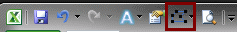
Click the arrow by the new button Edit Shape on your Quick Access Toolbar.
A short menu appears. Problem: The Edit Shape button is not active.
You did not click on the border of the comment to select it.
Solution: Right click on cell G1 and click on Edit Comment. Click the border of the comment to select the box.
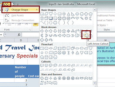
- Hover over Change Shape.
The palette of shapes appears.
-
 Experiment: Shapes
 There is no Live Preview when
you hover over a shape in the palette.
There is no Live Preview when
you hover over a shape in the palette.
- Click an interesting
shape.
Does your text fit?
Can you resize the shape so that the text does fit nicely? - Try out other shapes.
Notice that the resizing handles form a rectangle but the border of the shape may not touch that rectangle at all.
Older Shapes Palette: The shapes on this palette are not quite the same as the palette for AutoShapes. They seem to be an older version. In particular, in Excel 2013 and 2016 the symbol for an adjustment handle is a yellow diamond that Excel 2010 uses. Unexpected!
Text and Shape: Some shapes do not work well with text. Some shapes do not work well with the transparency. The fill color becomes quite dark and the lighter color shows only as part of the 3D effect. Of course you could change the font color to a light color if you really wanted the shape.
When you are ready to continue...
- Click an interesting
shape.
-
 Select the shape Left Arrow Callout in the Block Arrows section.
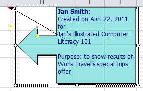
There is still an arrow pointing from the center of the rectangle to the cell where the comment is attached. Looks rather odd! This choice is not quite as attractive as it could be.
- Drag the bottom edge of the shape down to about the
bottom of row 4 to make it large enough to show all
of your text.
- Save.
[trips31-Lastname-Firstname.xlsx]
|
|
| © 1997-2017 Jan Smith All Rights Reserved |
Site Map What's New |
Privacy Policy Terms of Service Copyright Acknowledgements |
~~ 1 Cor. 10:31 ...whatever you do, do it all for the glory of God. ~~
Last updated: March 22, 2017