Jan's Working with Numbers

Format: Cells: Table Styles

Excel makes it easy to format part of your sheet as a table by providing a number of table styles.

Table Styles

The initial table styles have formatting for heading rows, borders, and alternating background colors for data. The colors are those in the document's current theme.

Apply a table style: Table Styles Gallery
Select the cells that you want to be in the 'table' first. Select a style from the gallery of table styles. Excel adds arrows for each column when you apply a table style, but, happily, those arrows won't print. An arrow opens a menu of sorting and filtering options for the table based on that column.

At the bottom of the gallery is a command, New Table Style..., which lets you create a custom table style that can be used on other tables and even in other workbooks.

Remove a table style: Clear formatting

Hide the sort/filter arrows: With at least one table cell selected, on the Data ribbon tab, click the Filter button to turn it off. The column arrows go into hiding. Not an obvious thing to do!

There are times when you regret you ever started formatting. You want to start over with no formatting at all. Undo works if you are willing to back up. But Undo remembers only the last 100 actions. The Clear Formatting command on the Clear button will remove what the table style applied, but will not clear formatting that you applied yourself.

In older versions of Excel, what is now called a table was called a list.

Themes

If you change the workbook's theme, the colors and fonts change for the table styles.

Office 2010 has more pre-designed themes than Office 2007 has. Office 2013 and 2016 have the same themes but not the ones that previous versions had!

A custom theme that you created shows at the top of the gallery of themes. If you did the Working with Words lessons, you created one, Sun-Tahiti. Any custom theme is available for any Office document, not just the program you were in when you created it.

Note that the PowerPoint slide part of a theme can only be designed while in PowerPoint. For themes that you create and save in other programs, Office automatically assigns a slide design.

Step-by-Step: Table Styles

What you will learn:

to format with table style
to clear all formatting
to change theme

Start with: trips10-Lastname-Firstname.xlsx (saved in previous lesson)

If necessary, open trips10-Lastname-Firstname.xlsx
Save as trips11-Lastname-Firstname.xlsx in the excel project3 folder of your Class disk.

Format Cells: Table Style

It is usually helpful to use different formatting for the labels for columns and rows and for cells that show totals. Excel has a large number of table styles, which use the theme colors and fonts to help with this. A 'table' in Excel is not just the whole spreadsheet, and it is quite different from a 'table' in Word.

Select the range A4:E25, which is the upper table on the sheet.
On the Home tab in the Styles tab group, click the button Format as Table.
The gallery of table styles opens.

How do these styles differ?
- Different colors from the document theme
- Format for header row different from data row
- Alternating color bands for rows
- Borders around rows or all cells, or no borders at all.
Live Preview does not work for the gallery from the Format as Table button to start with. But once you have applied a style, Live Preview does show the effect of the style your mouse is over.

New Style: The gallery of table styles includes a command for New Table Style... but such a new style will not show up later in the gallery for a different document. So sad... and annoying!
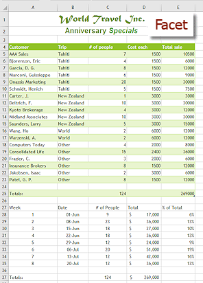
Select the style named Medium 2.
A dialog appears showing what cells will be in the table.
Be sure that the box is checked for My table has headers.
Click on OK.
The dialog closes, the style is applied to the table, the ribbon changes to the tab Table Tools: Design. The Table Styles gallery highlights the current table style.
What changes in the table itself?
- The header row gets down arrows for sorting.
- The data rows have alternating bands of background fill.
- The header row did not change formatting even though the color and font size are different from the Medium 2 table style.
Experiment: Table Style
With the table still selected, on the Table Tools: Design tab, hover over several different styles in the Table Styles gallery, but do not click(!).
Click the More button to see the full set of styles.

Live Preview shows you how the style you are hovering over would change the formatting of the table.

Examples:

The header row is not changing to match the style!
That is because earlier you applied formatting manually to those cells - font, font size, font color, fill color. For the table style to change cells that were already formatted, you have to remove that manual formatting.

When you are ready to continue...
Save
[trips11-Lastname-Firstname.xlsx]

Clear Formats

The Clear button on the Home tab has choices for what to clear, including just the formatting. That's just what you need right now. You did that manual formatting for row 4 a long time ago. Undo cannot help this time!

With the table still selected, on the Home tab in the Editing tab group, click on the Clear button.
The menu of choices opens.

Clear All will remove the formatting and the contents of the selected cells, too!
Click on Clear Formats.
The selection goes back to the default formatting for the sheet.
The arrows stay in the header row. The cells are still part of a 'table'.

Alternate Method: Right click on a table style thumbnail and select Apply and Clear Formatting.
This has the advantage of doing two things with one click!
Experiment: Table Style
- Try out several styles by hovering over a style in the Table Styles gallery on the Table Tools: Design tab.
  Now the header row changes with the table style.
  
  Examples:
Apply Medium 2 again.
The header row is similar to what you applied manually before, but the fill color is a bit lighter and the font size is smaller. You lost the accounting formatting for the totals in the last column.
Switch to the Data ribbon tab.
The Filter button is highlighted.
Click the Filter button.
The column arrows are hidden. The cells are still a table. You can get them back by clicking the Filter button again.
Save.
[trips11-Lastname-Firstname.xlsx]

Change Theme

The Themes gallery is big and hides a lot of your sheet. In Excel 2007 and 2010 you can use a smaller document window so you can see what Live Preview does to the document. But Excel 2013 does not have document windows inside the Excel window. It puts each document into its own window.

Excel 2007, 2010: Use a smaller document window
1. Click the Restore button for the document.
  This button is at the top right of the Excel window, below the controls for the Excel window.
  
  The workbook window resizes.
2. Drag the workbook window to the right to leave room at the left for the Themes gallery.
On the Page Layout tab, click on the Themes button.
A gallery of themes opens. You will have to scroll to see them all. Each version of Excel has a different set of themes.

If you have not done the Working with Words lessons, your gallery will not have the Sun-Tahiti theme that is in the illustration.
Experiment: Theme
Hover over but do not click on various themes to let Live Preview show what would change in your sheet.

Examples:

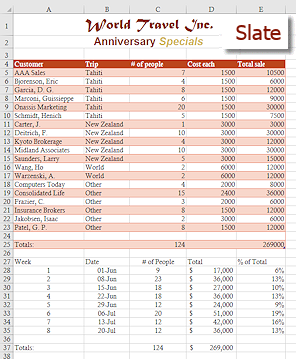
What changed?
- Fill colors for bands and header row
- Font and font sizes for cells
- Colors for titles (which were selected from theme colors)
What did not change?
- Fonts and font sizes that were manually applied (Title and subtitle)
- Font styles that were manually applied (Italics for 'Special')
- Alignment (Center in lower rows)
- Merged cells (Title and subtitle)
  
  When you are ready to continue...
If necessary, return the theme to Office .
Excel 2007, 2010: Click on the Maximize button for the worksheet window so that the window takes up all of the workspace again.
Save.
[trips11-Lastname-Firstname.xlsx]
Close the workbook.