
Jan's Working with Numbers
Format: Cells: Copy Formatting
Once you have decided on a formatting plan, you probably will want to use it on other cells. There are several ways to copy just the formatting. All methods apply to whole cells. If you want part of the text in a cell formatted differently, you will have to apply the formatting manually.
Animation: Format B3 and copy the formatting to other cells
| |
Step-by-Step: Copy Formatting |
|
| What you will learn: | to copy formatting with Format
Painter to copy formatting with AutoFill to copy formatting with Paste Special to resize columns to format only part of a cell's contents to apply a theme |
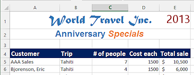
Start with: ![]() trips9-titleformatted-Lastname-Firstname.xlsx (saved in previous lesson)
trips9-titleformatted-Lastname-Firstname.xlsx (saved in previous lesson)
We will make things fancier using several different methods for copying formatting, just for practice. In the real world you would probably use only one at a time.
Format Cell: Format Painter
For quick copying of formatting, the Format Painter can't be beat!
- Select cell A4 = Customer
 From the
Home ribbon tab, select :
From the
Home ribbon tab, select :
Font: Calibri
Font Size = 14
Bold
Fill = Dark Blue (Standard colors)
Font Color = White
The row resizes automatically because of the larger font size.
-
 While cell A4 is selected, click on
 the Format Painter button.
The selected cell gets a blinking border. The pointer changes to the Format Painter shape.
-
 Click on cell B4 = Trip .
(Don't drag this time! That will apply the formatting to all cells that you drag over.)
The formats from cell A4 are applied to cell B4 and the pointer returns to the Select shape.  Save As trips10-Lastname-Firstname.xlsx on your Class disk in the excel project3 folder.
![]() Keep Format
Painter active: To use Format Painter
on several cells in different places, double-click the
Format Painter button. The pointer will stay in the Format Painter shape
until you click the button again or press the ESC key. Then the
pointer will go
back to the Select pointer shape.
Keep Format
Painter active: To use Format Painter
on several cells in different places, double-click the
Format Painter button. The pointer will stay in the Format Painter shape
until you click the button again or press the ESC key. Then the
pointer will go
back to the Select pointer shape.
![]() Copy formatting
for a range: Format Painter is smarter than it used to be.
You can copy the formatting for a whole range and apply it to a range
that is the same size or smaller. If the range is larger than the original range, the pattern of formats will repeat
across the new range.
Copy formatting
for a range: Format Painter is smarter than it used to be.
You can copy the formatting for a whole range and apply it to a range
that is the same size or smaller. If the range is larger than the original range, the pattern of formats will repeat
across the new range.
Format Cell: AutoFill
AutoFill is great for filling in a series of data but you can also use this feature to copy just the formatting.
- With B4 selected, move the mouse pointer over the bottom right corner of
the cell until the pointer changes to the AutoFill shape, a black cross
 .
.
-
 Drag to the right until the next two cells are selected.
The screen tip is showing that you are going to copy Trip into each of these cells. Don't panic yet!
-
Release the mouse button.
 Cells C4 and D4 look
exactly like B4. That's not
what we want, of course. Not to panic!
Cells C4 and D4 look
exactly like B4. That's not
what we want, of course. Not to panic!The AutoFill Options button
 shows at the bottom right of the filled cells.
-
 Hover over the AutoFill Options button to show its arrow.
- Click the arrow to open this menu.
- Click on Fill Formatting Only.
 The
cell text goes back to the original but the formatting now matches cells A4 and
B4.
The
cell text goes back to the original but the formatting now matches cells A4 and
B4.
Slick trick! - Save.
[trips10-Lastname-Firstname.xlsx]
Format Cell: Paste Special
The
Paste Special dialog can handle several different ways to 'paste'. You can
choose whether to paste everything or just the formula or just the current
calculated value or just the formatting or a combination of some of these.
-
 Select cell B4 and click
 the Copy button
on the Home tab.
the Copy button
on the Home tab.
The cell gets bordered with a blinking dashed border. The dashes look like they are chasing each other around the cell! - Click in E4.
 On
the Home tab, click the arrow below the Paste button to
open its menu.
On
the Home tab, click the arrow below the Paste button to
open its menu.
The menu uses icons to show what can be pasted and in what format. Is it clear to you what each one will do?
 Problem:
Paste button menu is different
Problem:
Paste button menu is different
You must copy something first.
Solution: Click on B4 again and then on the Copy button. Click on E4 and then on the Paste button arrow.
-
 Experiment: Paste options
 Excel 2007: Try a choice in the list of Paste options. Undo and try another choice.
Did the name of the choice make it clear what would happen?Did you guess right about each one? Some choices only affect numbers, not text.
Excel 2007: Try a choice in the list of Paste options. Undo and try another choice.
Did the name of the choice make it clear what would happen?Did you guess right about each one? Some choices only affect numbers, not text.

 Excel 2010, 2013, 2016: Hover over each icon in the Paste menu. Guess what will happen.
Live Preview changes cell E4 to show you what that choice would do. A screen tip tells what Paste would do.
Did you find one that will apply just the formatting to E4? There is one but don't use it this time.
When you are ready to continue...
-
 Select Paste Special… at the bottom of the menu.
The Paste Special dialog opens. This dialog has more choices! - Inspect the choices.
Each of these can be helpful in certain situations.
- Click on the Paste option Formats. Then click OK.
All of the formatting in cell B4 is applied to E4.
-
 Press the ESC key
to clear the blinking border around cell B4.
Press the ESC key
to clear the blinking border around cell B4.
- Save.
[trips10-Lastname-Firstname.xlsx]
Resize: Columns
Notice that the row got taller when the text got a larger font size but the columns did not resize. The labels look crowded and C4 is cutting off some of the text. Let's fix that now.
-
 Drag across the column headings C, D, and E .
-
 Double
click on the right edge of the column heading of one of the
selected columns.
Double
click on the right edge of the column heading of one of the
selected columns.
All the selected columns are resized with AutoFit to be wide enough to read all the characters. Now the text in C4 shows completely. - Save.
[trips10-Lastname-Firstname.xlsx]
Format Cell: Part of Cell Text
Sometimes you want part of the text in a cell to be formatted differently - color, italics, bold, font size, font,... whatever.
-
 Double-click cell A2 to get into Edit mode.
The Status bar should show Edit. - Select the word Specials and click
 the Italics button.
 - While "Specials" is still selected, change the Font color to Accent 2.
The colors are somewhat different in the various versions of Excel.  Click a different cell to save your change and
remove the selection.
Click a different cell to save your change and
remove the selection.- Save.
[trips10-Lastname-Firstname.xlsx]
Apply a Theme
A theme sets the default colors, fonts, and effects for objects. Changing a theme automatically updates your whole document IF you originally chose from the colors, fonts, and effects that were in the default theme. Colors that you applied from Standard or custom colors will NOT change with a new theme.
For this sheet you have used theme colors for the title and subtitle. But you applied fonts to the title and subtitle that are not theme fonts. For the cells in row 4 you kept the theme font but applied a background color that is not a theme color. So what will change and what will remain the same when you apply a new theme? Let's find out!
-
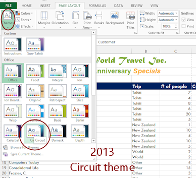
On the Page Layout ribbon tab, click on the Themes button to open the gallery of themes.
The current theme is Office and is highlighted.Be aware that the themes are different in different versions of Excel.
The opened gallery hides most of your cells. You can make a temporary change to the sheet so that Live Preview can show you what each theme will do.
- Resize column A to the right to at least 400 pixels and release.
 Open the Themes gallery again.
At least part of the titles and several columns should be visible to the right of the themes palette.-
Hover over each theme.
Scroll if necessary to see all of the theme thumbnails.What changes? What stays the same?
Some themes may actually use the current fonts and colors so you need to check out many themes to be sure. -
Undo any changes.
Keep in mind when you design your own spreadsheets that using theme colors and fonts lets you change the look of the whole workbook at once. Since you can create your own themes, there is no reason not to take advantage of this feature!
In the next lesson you will work more with themes after learning about table styles.
|
|
| © 1997-2017 Jan Smith All Rights Reserved |
Site Map What's New |
Privacy Policy Terms of Service Copyright Acknowledgements |
~~ 1 Cor. 10:31 ...whatever you do, do it all for the glory of God. ~~
Last updated: March 22, 2017