Jan's Working with Numbers

Exercise Excel 4-1:

Amazon Pings: Insert and Repair

---

What you will do:

Copy and insert data Paste Link Paste Formats Repair formulas Revise chart Print grouped sheets

---

Start with: , ex3-3-amazon-Lastname-Firstname.xlsx from Project 3: Ex. 3-3

Were your formulas in ex3-3-amazon-Lastname-Firstname.xlsx correctly designed to automatically include inserted columns? You will find out now.

1. Open ex3-3-amazon-Lastname-Firstname.xlsx from the excel project3 folder of your Class disk.
2. Save As with the name  ex4-1-amazon-Lastname-Firstname.xlsx  to the folder excel project4.
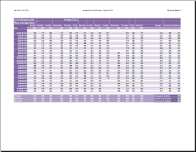
3. Select the sheet Week 2.
4. Copy A31:M33. Switch to a blank sheet and click in cell A1. Paste Values and Source Formatting.
   You will need these values later to see if they change when you add some new columns. Name this sheet Copy.
5. Insert Cells and Paste Link: Switch to the sheet Original Data and select the data for the third week (range Q1:W33). Copy. On sheet Week 2 click cell J1 and Insert Copied Cells. Shift cells to right. This inserts the cells but they are not linked to the original data, so paste again with Paste Link. (If you can not paste, the Clipboard lost your copy. Copy again from Original Data.)
   
   Why this awkward method? Inserting first creates the columns to Paste Link in. If you try to link first, you lose the existing columns for Average, Maximum, and Minimum.
6. Edit: Change cell G1 and the sheet tab to read Weeks 2 & 3. Remove the zeros from the cells that were originally blank. The data cells with zeros mean that the system was down at those times and no pings were recorded. Delete those zeros from Tues. and Wed. of Week 3 also since they are not real ping times. The Minimum time can not really be zero!
7. Copy table formats: Select column I and Copy. Select columns J through Q and Paste Formats.
8. Resize: AutoFit the new columns.
9. Check Formulas: Are all your formulas at the right end of each row including the new cells? Ranges should go to column Q.

10. Repair Formulas: Show the formulas. [CTRL + `] If necessary, revise the range for each formula in R6:T6 to go to column Q. Use AutoFill to copy the revised formulas down the column.
    Use the AutoFill Options button to Fill Without Formatting.

    Edit the formulas in T31:T33 to also go through column Q.

    If the autofilled cells are all the same, press the F9 key to make the sheet recalculate the formulas and show the new values.

    Compare cells T31:T33 with the values on the sheet Copy. They should be VERY different.

    [The totals will not automatically update when the formulas do not include the blank column, originally Column J.]

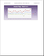
11. Chart: Edit the title for the chart to read  Amazon Pings - Weeks 2 & 3  and the sheet tab to read Chart - Weeks 2 & 3. Drag the updated chart wide enough to show all the dates along the bottom. (about as wide as columns A to L) The legend should still show Average, Maximum, and Minimum.

    [If the chart was not updated, then your original ranges for the chart did not include the blank column, Column J. Select the chart and right click on it. From the context menu choose Select Source Data…. Edit the ranges for Values for each Series and for Category (X) axis labels to end in column Q instead of column I.]

    [If the legend says Series 1, Series 2, and Series 3, right click the chart and choose Select Data. In the left part of the dialog, click on Series 1 and then on the Edit button. Change the name of the series to Average. Repeat for each series.]

12. Prepare to print: Edit the headers for the sheets to read Exercise Excel 4-1. Spell Check. Look at Page Break Preview and Print Preview. Select sheet Weeks 2 & 3, and on the Page Layout ribbon tab, set the orientation to Landscape and Scaling to Fit to 1 page wide by 1 page tall. Select sheet Chart - Weeks 2 & 3,  and on the Page Layout ribbon tab, check that it will print with Portrait orientation and Fit to 1 page wide by 1 page tall.
13. Save.  
    [ex4-1-amazon-Lastname-Firstname.xlsx] 
14. Select the two sheets Weeks 2 & 3 and Chart - Weeks 2 & 3.

15. Print the active sheets. One will be landscape and one portrait.
    [If the chart is still selected when you try to print, the chart will take up a whole page!]
    

    After the printing is finished, close the workbook.