Jan's Working with Numbers

The worksheet on tickets sold needs to be cleaned up. There is a lot of repeated data that can be managed more efficiently.

Start with: , ex3-1-theatertickets-Lastname-Firstname.xlsx (from previous exercise), tickets2-transparent.gif from resource files

1. Open the workbook ex3-1-theatertickets-Lastname-Firstname.xlsx  in the excel project3 folder of your Class disk.
   
2. Save as ex4-2-theatertickets-Lastname-Firstname.xlsx  to your Class disk in the excel project4 folder.
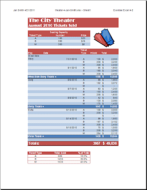
3. Insert image: Insert the image tickets2-transparent.gif from your resource files at the right of the Seating Capacity table, sized so that it is about the same height as that small table. Drag the resized image so that it is about in the center of the white area both horizontally and vertically.
4. Redundant data: Delete column D, price of the ticket. This data is also in the small upper table of ticket types. The formulas in the Total column will break - #REF!
   

5. Repair the formulas: Rewrite the formula in E11 to multiply the number sold in D11 by the price per ticket in the Seating Capacity table in C6. Use an absolute reference for the ticket price cell, C6. Similarly, correct the formulas for the next two cells for the B and M types of tickets.

   Recall that there is a pattern to the tickets, each performance has the same 3 types. Select E11:E13 and copy. Paste the formulas to the remaining rows of tickets sold. [Skip the subtotals rows!] You should get the same values in the Total column as before.
   

6. Extend the formatting for the title rows to column E.
   
7. Image: Adjust the position of the image to center it in the white space in columns D and E.

8. Format groups: Change the formatting of the subtotals for each play to Background Fill: Blue, Accent 1; Font color: White

   Format the grand total row: Background Fill: Accent 2, bold, not italics, Font size = 14; Font color: White.
   

9. Header: Change the header to show Exercise Excel 4-2.
10. Open Print Preview and look for errors. Correct any errors.
    
11. Print the sheet Sheet1.
    

12. Save.
    [theater4-Lastname-Firstname.xlsx]

    Next steps create a PivotTable to get a total for each type of ticket sold automatically, without having to select the subtotal cells.
    

13. Select C10:D36, the cells about ticket types and number of those tickets sold.
    

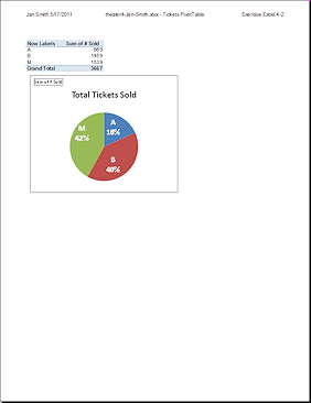
14. PivotTable: Create a PivotTable on a new sheet. Name the sheet Tickets PivotTable.
    Drag Ticket Type to the Row Labels area. Drag # Sold to the Values area.
    If necessary, change the Values to use SUM instead of COUNT.
    

    The (blank) row in the PivotTable represents the subtotal rows in Sheet1. Whoops. You cannot select just the cells you want. They are not adjacent. You could copy the data table and delete the subtotal rows, but it is easier to just filter this one!
    

15. Filter: Drop the list for Row Labels and uncheck the box beside (blank). Close the list.
    On the sheet you can see the Filter icon but Print Preview does not show this icon so you cannot tell that the data was filtered.
    
16. PivotChart: Add a PivotChart on the same sheet as the PivotTable.
    Use the first Pie chart type. Select a Layout that shows the % and the type without showing a legend.
    Move the chart to the far left and resize to make it close to square.
    Change the data labels to white, bold, and 16 pt.
    
17. Header: Setup the sheet header - name and date on the left, workbook and sheet in the middle, Exercise Excel 4-2 on the right. (Be sure the chart is not still selected!)
    
18. Print the sheet Tickets PivotTable.
    
19. Save.
    [theater4-Lastname-Firstname.xlsx]