Jan's Working with Numbers
Formulas: Exercise Excel 4-3

 You
will create subtotals for an existing sheet from the resource files about
subscriptions to Computers Today using the Subtotals feature and
manually. You will also create a PivotTable and PivotChart.
Exercise Excel 4-3: |
Computers Today: Subtotals |
| What you will do: | Sort Create subtotals with Subtotals button Create subtotals by hand Format groups with styles Insert image Create and edit a PivotTable and PivotChart |
The newsletter Computers Today ran special advertising in June. They want to look at the new subscriptions that came in that month to see if their ads had an effect. You will create a spreadsheet that will subtotal the new subscriptions by country.
Start with: ![]() , subscribers.xls and computer.gif in the resource files
, subscribers.xls and computer.gif in the resource files
- Open subscribers.xls from the numbers folder in the resource files or download now. The default location if you downloaded the zipped resource files is c:\My Documents\complit101\numbers\
This start-up document is in an older file format. It will open in Excel 2007 and 2010 in Compatibility Mode with the title bar showing [Compatibility Mode]. This mode keeps you from using new Excel features. That's good if you need to be able to open the file later in an older version of Excel. It's bad if you want to use the new Excel features!
-
 Save as ex4-3-subscribers-Lastname-Firstname.xlsx to the excel project4 folder of your Class disk.
Be sure to change the file type to Excel workbook (*.xlsx). Do not just type the extension in. Be sure the File Type shows this extension.
- Copy the contents of Sheet1 to Sheet2.
Rename Sheet1 to Subtotals.
Rename Sheet2 to Original.
Steps below are for the Subtotals sheet:
-
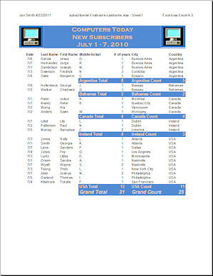
Title style and labels: Center each title line across the table columns (The cells are already merged.). Create a cell style named MyTitle with Copperplate Gothic Bold, Bold, font size 18, font color: an orange from the theme colors at Lighter 40%; fill color: a blue at Darker 25%. Apply this style to the title and the two subtitles.
Make the column labels in Row 5 Bold.
- Image: At the top left and right of the titles insert the
image of a computer from the resource files. Resize the image to the
height of rows 1, 2, and 3. (You can download just this
file, if necessary: computer.gif)
- Sort: Sort the table data on Country, City, and Last
Name.
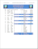
- Count Subtotals: Use the Subtotal command to create subtotals
for each country using the function Count.
-
Styles: Create a cell style named Subtotals: Arial, Bold, font color: an orange at Lighter 40%, Font size 11, fill color: a blue at Darker 25%. Apply it to all the country subtotals. (Be sure to check the Font box in the dialog for creating a new style.)
Create a cell style named Grand for the Grand Count: Arial, Bold, Italic, font size 14, font color: an orange at Lighter 40%; fill color: a blue at Lighter 40%,
If necessary, change the format for the subtotal cells to General.
 Sum Subtotals: In the # of Years column, create a sum for the
# of Years for each country and a Grand Total at the bottom. You can not
use the Subtotal command to do this because it can only use one
function. You cannot use Count and Sum at the same time with the
Subtotals dialog. You must create these sums yourself.
- Sum Labels: Add labels like "Argentina Total" to column D
for each country sum in column E.
- Format Sums: Use the Subtotal and Grand styles to format the
totals and labels you just created.
- Format columns: Center the data in the Date and # of Years
columns. Resize columns if necessary to show your labels for the new
totals. If necessary, move the computer image to the far right of the colored background at the top of the page.
- Header: Setup the sheet header - name & date on the left,
workbook and sheet in the middle, Exercise Excel 4-3 on the right.
-
 Save.
Save.
[subscribers4-Lastname-Firstname.xlsx]
-
 Print the sheet Subtotals.
Next steps create a new sheet: PivotTable
-
 Switch to the sheet Original and select all the data cells,
A5:G30.
-
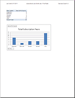
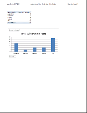
PivotTable: Create a PivotTable in a new sheet. Rename the sheet as PivotTable.
Use the Country field for the rows and # of years for the Values.
- Create a PivotChart.
- Edit PivotTable and PivotChart:
If necessary, apply a PivotTable style that colors the top and bottom rows of the pivot table.
Remove the legend from the PivotChart.
Change the chart title to "Total Subscription Years".
- Header: Setup the sheet header - name and date on the left,
workbook and sheet in the middle, Exercise Excel 4-3 on the right.
-
 Save.
Save.
[subscribers4-Lastname-Firstname.xlsx]
-
 Print the sheet PivotTable.

This exercise uses files from the numbers resource files.
The default location for these files is c:\My Documents\complit101\numbers\ Save the changed document to your Class disk in the excel project4 folder. This keeps the original files intact in case you need to start over or another student will be using this same computer.