 |
There are several different ways
of viewing an Excel worksheets. Each helps you work in different situations.
Three are found on the View menu. (Logical, huh!) Two are on the Window menu
and one more on the File menu. In addition Zoom works in all the views to enlarge
or reduce what you see on your screen.
View Choices
-
 Normal - the default view, which shows gridlines
and headings for columns and rows.
-
 Page Break Preview - a reduced view of the sheet
with blue lines marking where breaks will occur and what will actually print
if you print the sheet. Gridlines and headings are still shown. Unlike word
processors, Excel will let you block out part of a sheet so that it won't print.
-
 Full Screen - hides everything on the screen but
the sheet itself. No toolbars or menu.
-
 Print Preview - shows how sheet will look on paper.
Available on the File menu and as toolbar button.
-
Split - divides the screen into
four panes, so you can view different parts of a large sheet at the same time.
Found on the Window menu. Or, you can create just two panes by dragging the
Split box on a scrollbar.
-
Freeze Panes - fixes part of
the sheet in place while allowing the rest of the sheet to scroll. This lets
you keep the column and row headings in view.
|
 |

Where you are:
JegsWorks >
Lessons >
Numbers
Before
you start...
Project 1: Excel Intro
Interface
Select & Navigate

 Select
Cell Select
Cell
 Select
Range Select
Range
 Select
Row/Column Select
Row/Column
 Select
Sheet Select
Sheet
Methods

Shortcut keys

 Views Views
Common Tasks
Summary
Quiz
Exercises
Project 2: Excel Basics
Project 3: Format & Arrange
Project 4: Groups & Formulas
Project 5: Design
Search
Glossary
Appendix |
|

|
Step-by-Step: Views
|
 |
|
What you will learn:
|
to switch to a different view
to keep part of a sheet from printing
to toggle Full Screen on and off
to split the view into 4 parts
to split the view into 2 parts
to freeze panes to keep column and row titles in view
|
Start with:
 (Excel
open to budget.xls from resources) (Excel
open to budget.xls from resources)
View: Normal
- If necessary, select | from the menu.
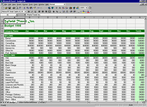
 The Normal View displays the document with the
grid lines in gray. This is the default view. In Normal you may see a dotted
line between rows or columns to show where page breaks fall. Such a line
is hard to see and only show after you have looked at the Print
Preview.
View: Page Break Preview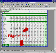
- Select from the menu |
.

 The Page Break Preview displays wide blue lines around the parts of the
worksheet that will print on the same page.
 Pages are labeled with large gray numbers (that won't print) in the center
of each page area so you can see what order the sections of the worksheet
will print. For large sheets with many rows and columns, it can get confusing
as to what parts will print with what. Pages are labeled with large gray numbers (that won't print) in the center
of each page area so you can see what order the sections of the worksheet
will print. For large sheets with many rows and columns, it can get confusing
as to what parts will print with what.
-
 Drag
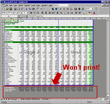
the bottom blue line up underneath Row 42- Wages. Now the last 3 rows won't
print. Drag
the bottom blue line up underneath Row 42- Wages. Now the last 3 rows won't
print.
The Print Area (the part that will actually
print) shows cells with a white background. Areas that will not print have
a dark gray background. You can also set the Print Area using the menu
| .
While viewing the Page Break Preview, you can edit the cells, move the
blue boundaries, and resize columns and rows to make the results clearer.
For example, in budget.xls you might want to drag the blue borders
and insert new ones to so that the columns for each quarter would print
on a separate page.
- Switch back to Normal view using the View menu.
View: Full Screen
-
  Choose from the menu |
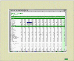
Full Screen shows more of the sheet by hiding the toolbars, scrollbars,
and other window parts. The Menu bar is still there as well as the Windows
taskbar.

- Click the Close Full Screen button, which will be floating
or else docked at one of the screen edges. You return to your previous view,
which was the Normal view if you are following the directions closely.
View: Print Preview
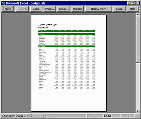
- Click on
 the Print Preview button on the toolbar.
This view shows the pages as they will be printed. Notice that the rows
aren't showing that had gray background in the Page Break Preview.
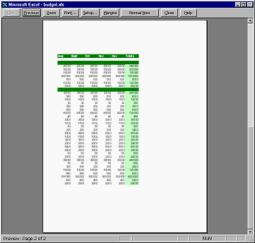
- Click on the Next button to see the second page that will
be printed. The Next button turns gray and the Previous button turns
dark.
- Try out the some of the buttons but do not Print. The total number
of pages is on the status bar with the current page number.
- Zoom - toggles between a full page view
and a 100% view.
- Margins - toggles margin lines on and off.
You can drag the lines to adjust margins.
- Setup - opens the Page Setup dialog, which
is also on the File menu. Excel has a more flexible shrink feature on
the Page tab of the Page Setup dialog.
- View button - will show either Normal View
or Page Break Preview, the one you were not in last.
- Close - does not close the documents but
instead closes the preview. You return to the view you just left.
- Unlike Word, there is no ruler and no Shrink to Fit button.
- Close this view by clicking the Close button on the bar.
View: Split
-
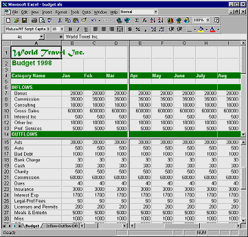 From
the menu select |
. From
the menu select |
.
A Split View of 4 panes is created. You can drag the bars to resize
the panes.
- Remove the splits with the menu command | .

- Drag the Split boxes on the vertical and horizontal scroll
bars to create other split views. (Watch out! There is similar box at the
end of the sheet tabs which resizes the space for tabs.)
New scrollbars appear for each split. Such splits are useful when you
need to see widely separated sections of the sheet at the same time. A selected
cell or range will show as selected in any pane in which it is visible.
- Use each scrollbar to see which panes scroll with which
scrollbars.
- Remove the splits by dragging the split boxes back to
their original positions, or use the command on the Window menu.
View: Frozen panes
Frozen panes do not scroll while the rest of the sheet
does. This effect is used primarily to hold labels for the rows or columns
in place while you scroll to the part of the sheet you are interested in.
Without the labels it can be hard to tell what you are looking at.
- Select row 5. Then select | . The rows
above your selected row are frozen. A dark line will appear at the
edge of the frozen pane.
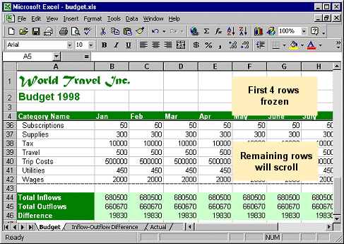
- Scroll up and down. The top four rows of the sheet stay put!
- Unfreeze the pane with |
.
- Select Column B and then | . The
columns to the left of your selected column are frozen.
- Scroll left and right. The first column remains in place.
- Unfreeze the pane.
- Select cell B5 and the | . The
rows above and the column to the left are frozen.
- Scroll up and down and also left and right. The top and left
of the sheet remain in place so you can see the labels. Very useful on large
sheets.
- Unfreeze the panes.
|

![]()