 |
Creating and applying styles is
rather awkward with the Style Dialog. Using a toolbar control would be easier.
For some reason Excel does not include the Style Box on the default Formatting
bar like Word does.
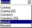 First you will learn how to add this control to a toolbar.
Then you will create and apply styles with the Style Box. First you will learn how to add this control to a toolbar.
Then you will create and apply styles with the Style Box.
|
 |

Where you are:
JegsWorks >
Lessons >
Numbers
Before
you start...
Project 1: Excel Intro
Project 2: Excel Basics
Project
3: Format & Arrange
Format Cells

 Apply
Formatting Apply
Formatting
 Copy
Formatting Copy
Formatting
 Partial,
AutoFormat Partial,
AutoFormat
 Style
- Dialog Style
- Dialog
 Style
- Style box Style
- Style box
Format Chart
Arrange
Summary
Quiz
Exercises

Project 4: Groups & Formulas
Project 5: Design
Search
Glossary
Appendix |
|

|
Step-by-Step: Cell Style Box
|
 |
|
What you will learn:
|
to customize a toolbar
to restore a toolbar
to apply a style with the Style Box
to create a Style with the Style Box
to show and print formulas
|
Start with:
 trips13.xls (saved in
previous lesson)
Toolbar: Customize
-
 Right
click on any toolbar. The popup menu of toolbars appears. The
ones with checkmarks are currently displayed. Right
click on any toolbar. The popup menu of toolbars appears. The
ones with checkmarks are currently displayed.
- If necessary, display the toolbar you plan to customize
by clicking on its name.
- Click on Customize at the very bottom of the menu. The
Customize dialog appears.
This command can also be found with | .
- Click on the Commands tab. This tab lists the categories
of commands on the left and the commands in each category on the right.
Each command can be placed on a toolbar or in a menu.
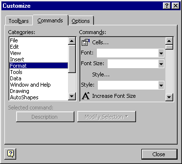
- Click on each category on the left in turn and scroll
the list of its commands on the right. You may see several commands
that you wish were on a toolbar. Sadly, there is only room for so many at
a time.
- Select the Format menu, on the left.
- Drag the Style box from the Commands list up to Excel's
menu bar, or to the Formatting bar, if you have room on it.
- Drop it in the
blank area of the bar.
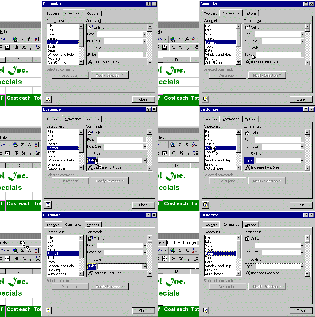
The Style box is now ready to use.
Excel will remember your toolbar from now on, unless your network
resets such things once you log out. Only the styles created
for the document or those in the underlying template will be in the list
- just like in Word.
If you are using a resolution larger than 640 x 480, you may have room
for this control on the Formatting bar, where it logically belongs. Add
other buttons if you like.
You can make more room on a toolbar by removing buttons that you don't
use much. Just drag a button to the Customize dialog and drop it. Then you
can drag a command you like to the toolbar in its place.
[If you are working on a network where you have your own password,
the computer should remember your settings. You can leave the toolbars the
way you like. If you don't have a password and are sharing the computer,
you may need to restore the toolbar. (See below) If you add and remove a
lot of buttons, the next user may get quite confused!]
- Click on OK to close the Customize dialog.
-
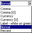 Open
the Style box list, that you just put on the toolbar, by clicking the down
arrow at the end of the box to see the short list of styles available.
Press ESC to close the list without applying a style. Open
the Style box list, that you just put on the toolbar, by clicking the down
arrow at the end of the box to see the short list of styles available.
Press ESC to close the list without applying a style.
Style: Apply with Style box
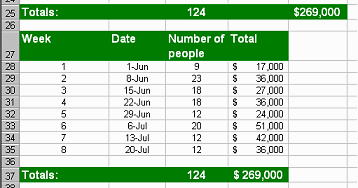
- Edit cell C27 to read Number of people
.
- Select ranges A25:E25, A27:D27, A37:D37.
(Hint: hold the CTRL key down while selecting.)
- In the Style box select the style Label-white
on green to apply it to the selected ranges. Wasn't that easy?
The cells you have styled have lost some formatting that had been applied
earlier.
-
 Center
cells C4, C25, A27:D27, and C37. Center
cells C4, C25, A27:D27, and C37.
- Select cells E25 and D37. Apply the Currency
style and Decrease Decimals twice.
- AutoFit Columns D and E again.
Style: Create in Style box
It is much easier to create and use a style when the Style
box is available.
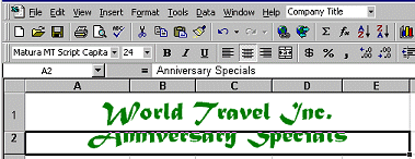
- Select cell A1, which is already formatted, of course.
- Click in the Style box you just added to the Menu bar.
- Type Company Title and press
ENTER.
- Drop the Style box list to see your new style.
 The style name is not displayed
using its formatting as recent versions of Word do. So name your styles in a way
that keeps it clear what they look like or what they are for. The style name is not displayed
using its formatting as recent versions of Word do. So name your styles in a way
that keeps it clear what they look like or what they are for.
- Apply your new style Company Title to cell A2 to
see if it does what you expected, but don't press Enter yet. Hmmm. Not very
helpful actually. Let's not apply this formatting after all.
-
 Click
Undo to return the cell to its previous state. Click
Undo to return the cell to its previous state.
- Open and check
Portrait orientation.
- If necessary, open and remove the page break.
-
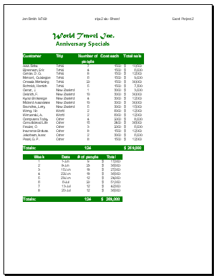 Open
Print Preview. Both tables should display on one page. Open
Print Preview. Both tables should display on one page.
-
 Save as trips14.xls to the
excel project3 folder on your Class disk.
 How to handle a full disk . How to handle a full disk .
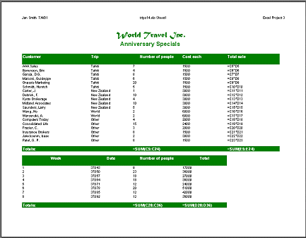
Print: Formulas
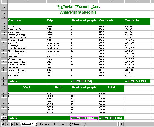
Sometimes you want to look at the formulas being used
in your cells without having to click on each cell. You might even need to
print this out so you can study what is going on.
- Select from the menu |
|
- Click on Formulas under Window Options. Click on OK.
The columns widen to display the full formula in each cell.
- Check your formulas. Are they all correct?
- Open to
the Page tab and change to Landscape Orientation.
- Switch to Page Break Preview and remove any page breaks
you find. Your sheet will actually fit on one page.
 If you
widen the column when you show formulas, when you return to showing values,
your columns will stay wide. If you leave the column widths alone, the sheet
will return to the exact state it was before showing formulas. If you
widen the column when you show formulas, when you return to showing values,
your columns will stay wide. If you leave the column widths alone, the sheet
will return to the exact state it was before showing formulas.
 Print.
-
 Switch back to showing values instead of formulas with
the key combo CTRL + `. (That's a left quote mark. On the English keyboard
this symbol is on the far left key of the row with the numbers keys.)
This key combo works to toggle the showing of formulas on and off. Of
course, you could also go back through the menu and uncheck the checkbox
you checked earlier. Switch back to showing values instead of formulas with
the key combo CTRL + `. (That's a left quote mark. On the English keyboard
this symbol is on the far left key of the row with the numbers keys.)
This key combo works to toggle the showing of formulas on and off. Of
course, you could also go back through the menu and uncheck the checkbox
you checked earlier.
- Switch the page orientation back to Portrait
| | .
-
 Save. [trips14.xls]
 How to handle a full disk . How to handle a full disk .
Toolbar: Restore
You don't need to do this next section if you are working
on your own computer, or if you are on a network with passwords that will
remember your personal settings.
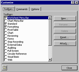
- To return a customized bar to the defaults, select
|
- Select the toolbar in the list that you changed and now
want to restore.
- Click on the Reset button. Then close the dialog.
-
 Save. [trips14.xls]
 How to handle a full disk. How to handle a full disk.
|

![]()